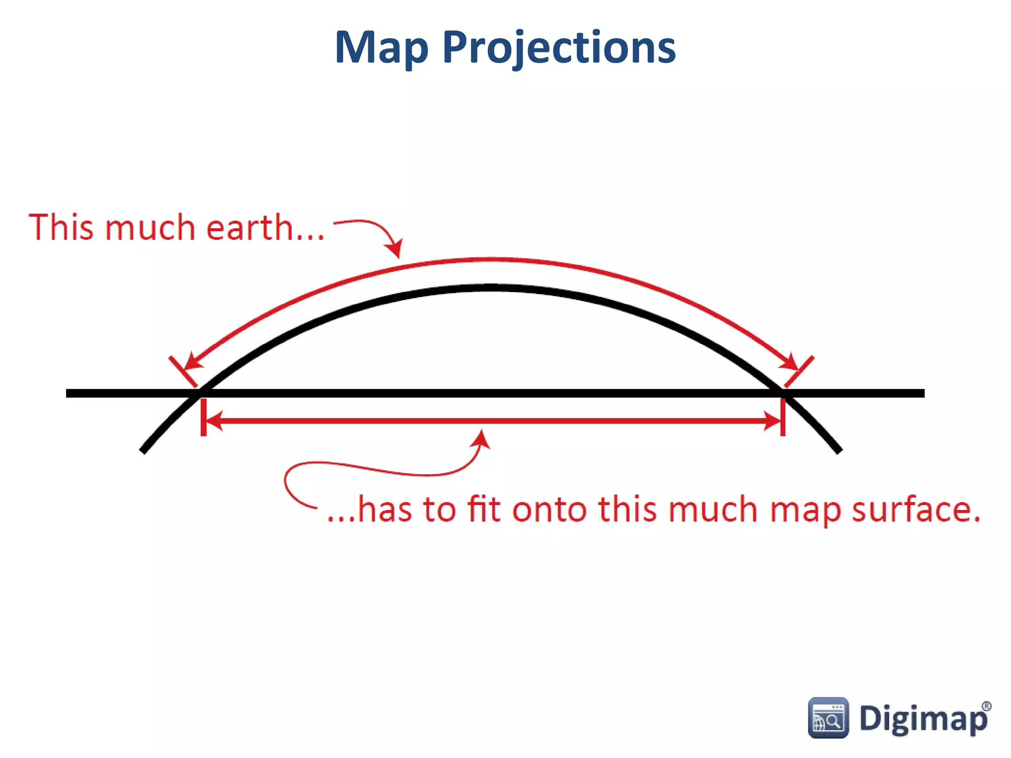
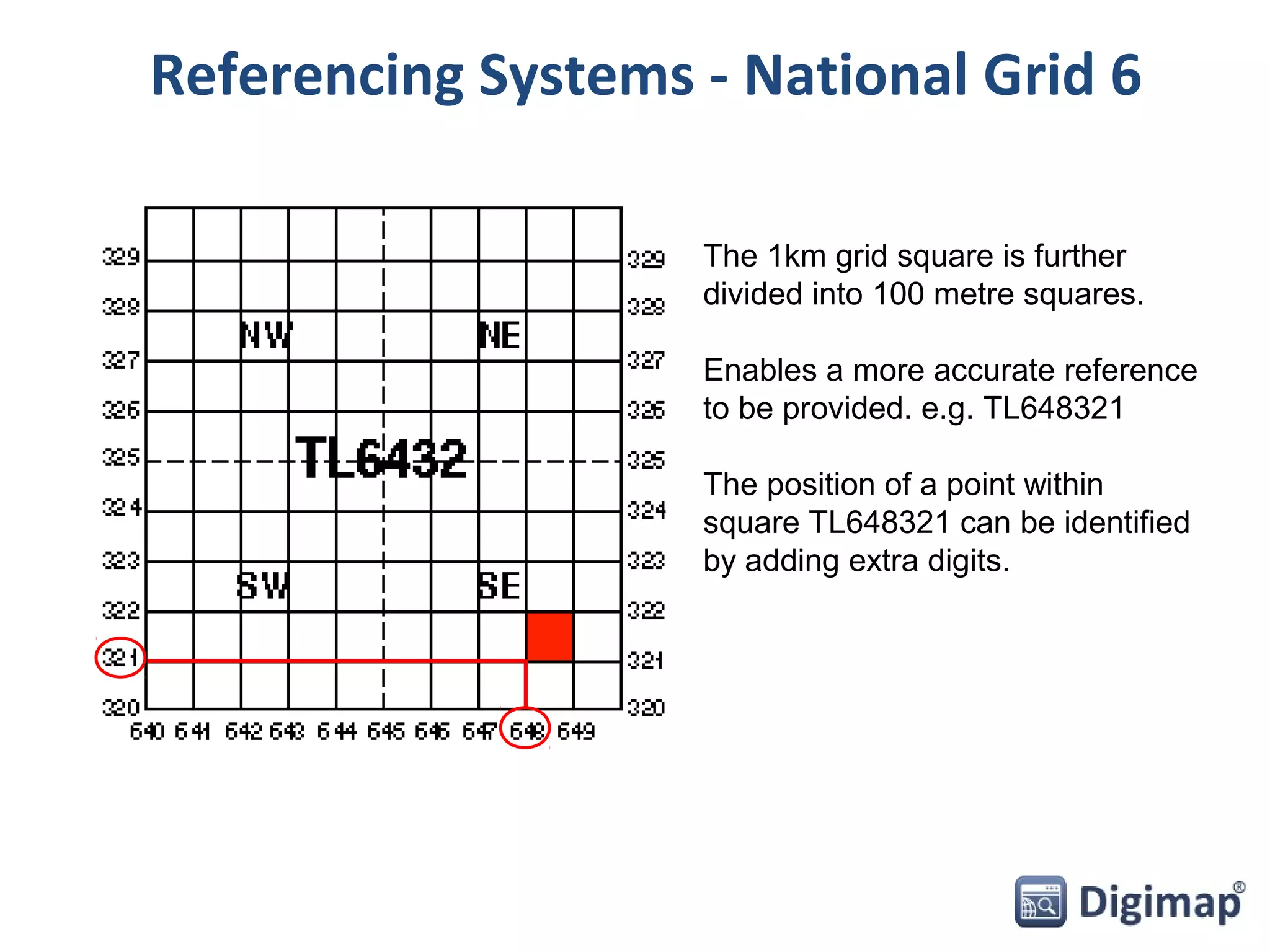
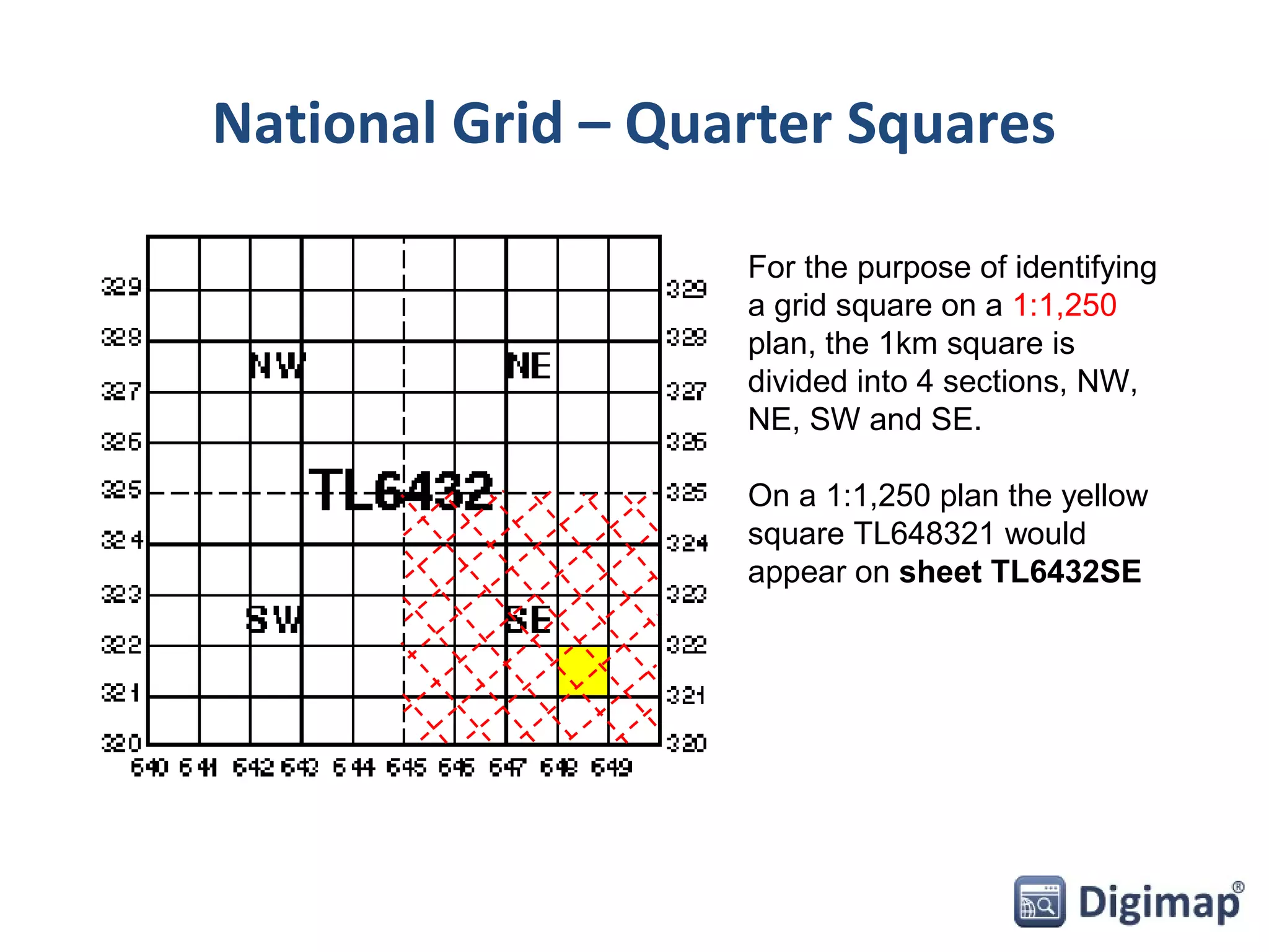
Cartographic Concepts 
Aim: to provide you with a basic 
knowledge of Cartographic Concepts
Objectives 
• By the end of this session you will: 
– recognise large and small scale maps 
– understand level of detail that can be shown at each 
scale 
– understand projections and coordinate systems 
– know why data in different projections need 
converting before they can be used together
Map Scales 
• any map is a scale representation of the Earth’s 
surface 
• scale may be defined as: 
– the ratio between distance measured on the map and the 
true distance on the ground
Map Scales 2 
• scale may be expressed in several ways: 
– as a Representative Fraction 
• e.g. 1:1,250; 1:250,000; 1:63,360 
• “One unit on the map represents 1,250 units on the 
ground” 
– in words 
• e.g. “one inch to one mile” 
• “One inch on the map represents one mile on the ground” 
– by scale lines 
0 50 100m
Map Scales 3 
• large scale or small scale? 
• relative terms: vary by subject 
• no absolute definition of large and small scale
Map Scales 4 
Contains Ordnance Survey data © Crown copyright and database right 2014
Map Scales 5 
• … remember it’s all relative!
Map Projections
Map Projections 2 
• a map projection transforms spatial relationships 
from a curved surface onto a flat plane using 
mathematical algorithms. 
• projections can be divided into 3 groups: 
Cylindrical Azimuthal Conic
Map Projections 3 
• GB Projection 
– O.S. use a cylindrical projection called Transverse Mercator 
– Origin is 49 degrees north and 2 degrees west 
• Just south of Jersey 
• Height Datum 
– Height information expressed as a measurement above a smooth 
assumed reference known as a Datum 
– usually Mean Sea Level at some point on coast 
• GB use Newlyn, Cornwall (Ordnance Datum) 
• France use Marseilles 
• Switzerland use Lake Geneva
Referencing Systems 
• to locate any point, feature or area on the Earth’s surface or a map 
it is necessary to have concepts and definitions of direction and 
distance 
• three main categories of referencing system: 
– Geographic (applies globally) 
• e.g. lines of latitude and longitude 
– Rectangular (applies locally) 
• e.g. Ordnance Survey National Grid system 
– non co-ordinate (applies locally) 
• e.g. Post Codes, Zip Codes
Referencing Systems 2 
• Ordnance Survey National Grid 
– based on the Transverse Mercator Projection 
– origin off-set by 100km North and 400km West to 
ensure that the U.K. is covered by positive co-ordinates 
– this origin is as far south as the Scilly Isles and as far 
west as St Kilda
Referencing Systems - National Grid 
Relationship between Transverse 
Mercator graticule and O.S. National 
Grid System. 
Red dot indicates true origin 49°N and 
2°W 
Green dot indicates false origin of GB 
National Grid, offset from true origin by 
100km north and 400km west
Referencing Systems - National Grid 2 
The UK is covered a by a 500 x 
500 km square grid. This is a 
remnant of a previous referencing 
system.
Referencing Systems - National Grid 3 
The grid is divided into 100 x 100km 
squares each identified by two letters. 
Note that the letter I is not used.
Referencing Systems - National Grid 4 
Each 100km grid square is 
divided into100 x 10km squares. 
These are from 0-9 from the SW 
corner left to right and from 
bottom to top. 
Using this system we can 
identify a 10km grid square 
e.g. TL63
Referencing Systems - National Grid 5 
The 10km grid square is divided 
into 1km squares 
Each is numbered as before 
from 0-9 
Used in conjunction with the 
10km grid square reference we 
can identify a 1km grid square 
e.g. TL6432 
6 
4 
3 
7
Referencing Systems - National Grid 6 
The 1km grid square is further 
divided into 100 metre squares. 
Enables a more accurate reference 
to be provided. e.g. TL648321 
The position of a point within 
square TL648321 can be identified 
by adding extra digits.
National Grid – Quarter Squares 
For the purpose of identifying 
a grid square on a 1:1,250 
plan, the 1km square is 
divided into 4 sections, NW, 
NE, SW and SE. 
On a 1:1,250 plan the yellow 
square TL648321 would 
appear on sheet TL6432SE
Conversion 
• Other data can be in different projections 
– Google = Web Mercator 
– GPS data = WGS 84 
– Different countries 
– Different zones 
• Different Conversions have different accuracies 
– Different GIS Software use different formulae 
– The default isn’t always the best
Conversion 2 
• OSGB_1936TOWGS1984_Petroleum 
– Best option “out of the box” 
• National Grid Transformation OSTN02 
– Most accurate option 
– Can be added to ArcGIS via OS website 
• Further Reading: 
– http://digimap.edina.ac.uk/webhelp/digimapgis/index.htm#pro 
jections_and_transformations/converting_between_osgb36_an 
d_wgs84.htm 
– http://www.ordnancesurvey.co.uk/docs/support/guide-coordinate- 
systems-great-britain.pdf

Mapping Projections and Data conversions

  • 1.
    Cartographic Concepts Aim:to provide you with a basic knowledge of Cartographic Concepts
  • 2.
    Objectives • Bythe end of this session you will: – recognise large and small scale maps – understand level of detail that can be shown at each scale – understand projections and coordinate systems – know why data in different projections need converting before they can be used together
  • 3.
    Map Scales •any map is a scale representation of the Earth’s surface • scale may be defined as: – the ratio between distance measured on the map and the true distance on the ground
  • 4.
    Map Scales 2 • scale may be expressed in several ways: – as a Representative Fraction • e.g. 1:1,250; 1:250,000; 1:63,360 • “One unit on the map represents 1,250 units on the ground” – in words • e.g. “one inch to one mile” • “One inch on the map represents one mile on the ground” – by scale lines 0 50 100m
  • 5.
    Map Scales 3 • large scale or small scale? • relative terms: vary by subject • no absolute definition of large and small scale
  • 6.
    Map Scales 4 Contains Ordnance Survey data © Crown copyright and database right 2014
  • 7.
    Map Scales 5 • … remember it’s all relative!
  • 8.
  • 9.
    Map Projections 2 • a map projection transforms spatial relationships from a curved surface onto a flat plane using mathematical algorithms. • projections can be divided into 3 groups: Cylindrical Azimuthal Conic
  • 10.
    Map Projections 3 • GB Projection – O.S. use a cylindrical projection called Transverse Mercator – Origin is 49 degrees north and 2 degrees west • Just south of Jersey • Height Datum – Height information expressed as a measurement above a smooth assumed reference known as a Datum – usually Mean Sea Level at some point on coast • GB use Newlyn, Cornwall (Ordnance Datum) • France use Marseilles • Switzerland use Lake Geneva
  • 11.
    Referencing Systems •to locate any point, feature or area on the Earth’s surface or a map it is necessary to have concepts and definitions of direction and distance • three main categories of referencing system: – Geographic (applies globally) • e.g. lines of latitude and longitude – Rectangular (applies locally) • e.g. Ordnance Survey National Grid system – non co-ordinate (applies locally) • e.g. Post Codes, Zip Codes
  • 12.
    Referencing Systems 2 • Ordnance Survey National Grid – based on the Transverse Mercator Projection – origin off-set by 100km North and 400km West to ensure that the U.K. is covered by positive co-ordinates – this origin is as far south as the Scilly Isles and as far west as St Kilda
  • 13.
    Referencing Systems -National Grid Relationship between Transverse Mercator graticule and O.S. National Grid System. Red dot indicates true origin 49°N and 2°W Green dot indicates false origin of GB National Grid, offset from true origin by 100km north and 400km west
  • 14.
    Referencing Systems -National Grid 2 The UK is covered a by a 500 x 500 km square grid. This is a remnant of a previous referencing system.
  • 15.
    Referencing Systems -National Grid 3 The grid is divided into 100 x 100km squares each identified by two letters. Note that the letter I is not used.
  • 16.
    Referencing Systems -National Grid 4 Each 100km grid square is divided into100 x 10km squares. These are from 0-9 from the SW corner left to right and from bottom to top. Using this system we can identify a 10km grid square e.g. TL63
  • 17.
    Referencing Systems -National Grid 5 The 10km grid square is divided into 1km squares Each is numbered as before from 0-9 Used in conjunction with the 10km grid square reference we can identify a 1km grid square e.g. TL6432 6 4 3 7
  • 18.
    Referencing Systems -National Grid 6 The 1km grid square is further divided into 100 metre squares. Enables a more accurate reference to be provided. e.g. TL648321 The position of a point within square TL648321 can be identified by adding extra digits.
  • 19.
    National Grid –Quarter Squares For the purpose of identifying a grid square on a 1:1,250 plan, the 1km square is divided into 4 sections, NW, NE, SW and SE. On a 1:1,250 plan the yellow square TL648321 would appear on sheet TL6432SE
  • 20.
    Conversion • Otherdata can be in different projections – Google = Web Mercator – GPS data = WGS 84 – Different countries – Different zones • Different Conversions have different accuracies – Different GIS Software use different formulae – The default isn’t always the best
  • 21.
    Conversion 2 •OSGB_1936TOWGS1984_Petroleum – Best option “out of the box” • National Grid Transformation OSTN02 – Most accurate option – Can be added to ArcGIS via OS website • Further Reading: – http://digimap.edina.ac.uk/webhelp/digimapgis/index.htm#pro jections_and_transformations/converting_between_osgb36_an d_wgs84.htm – http://www.ordnancesurvey.co.uk/docs/support/guide-coordinate- systems-great-britain.pdf