Downloaded 72 times

![분산시스템 연구실
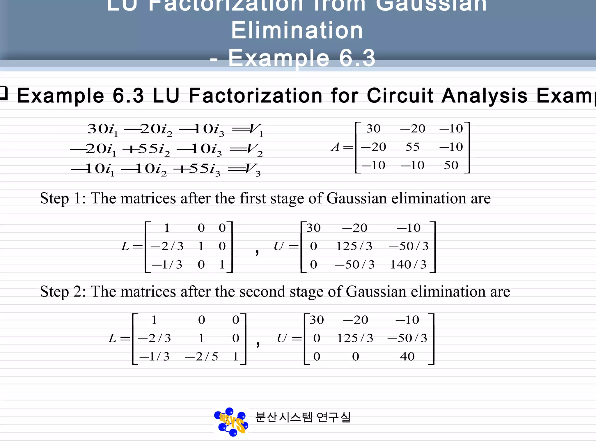
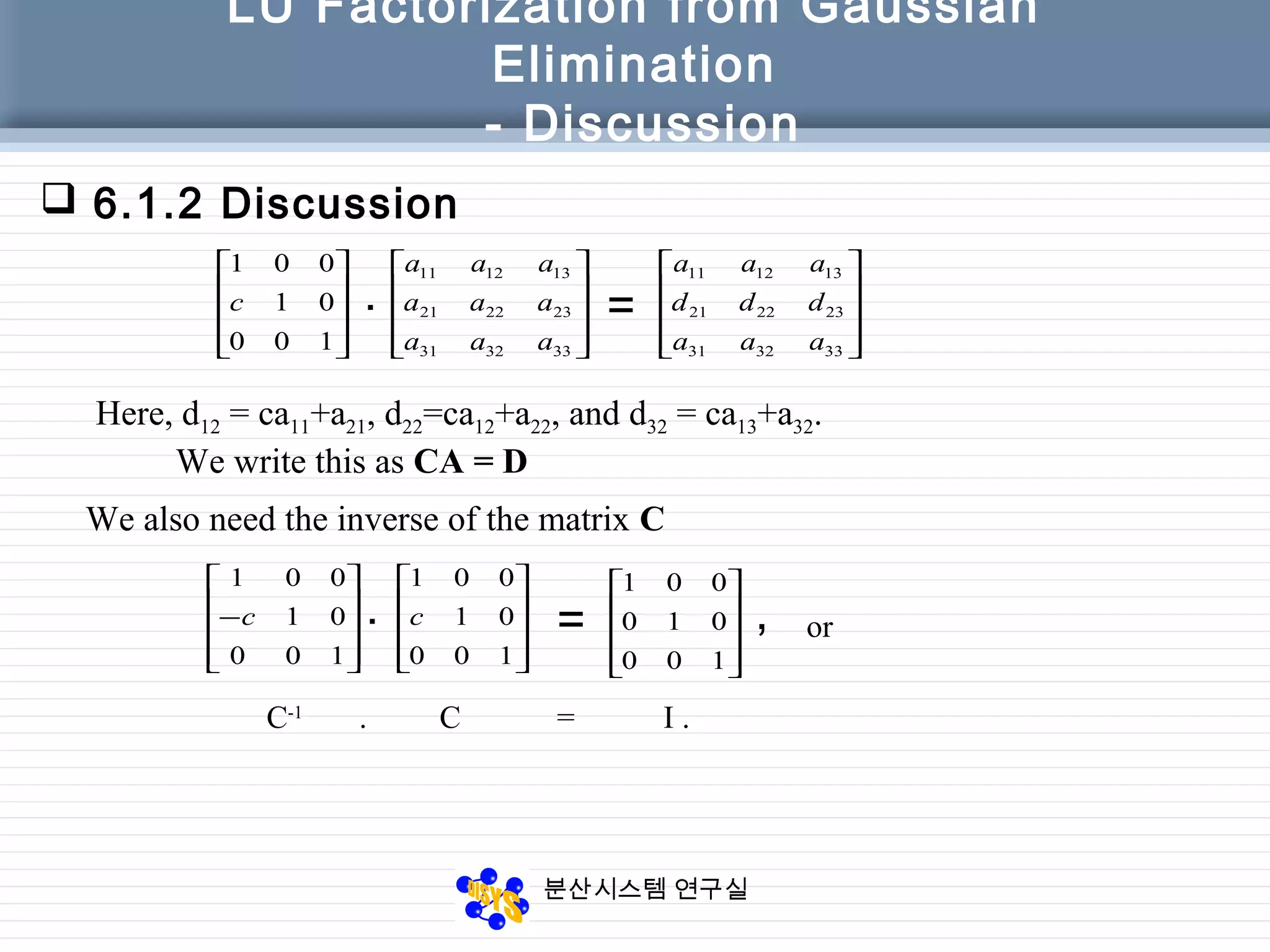
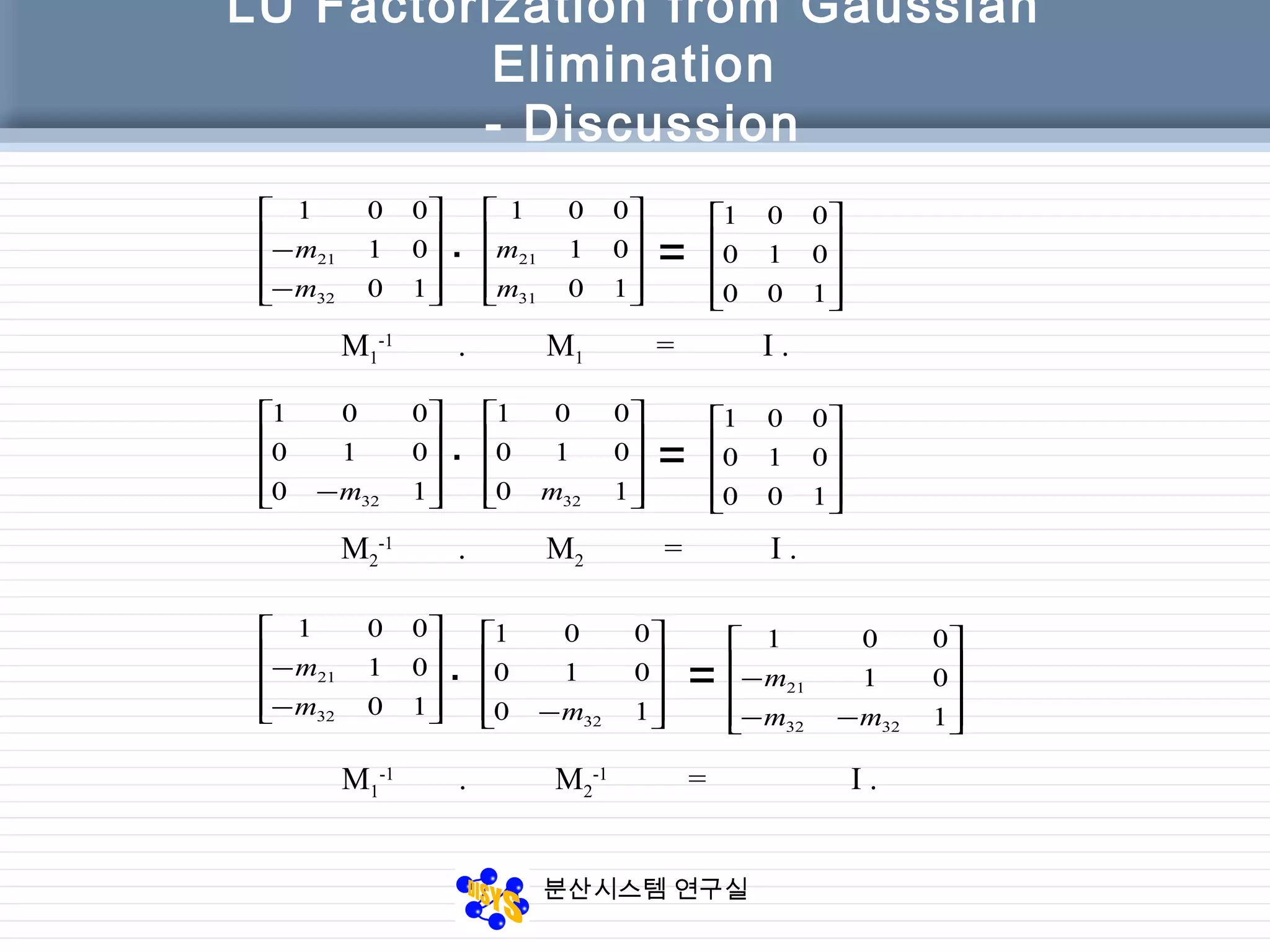
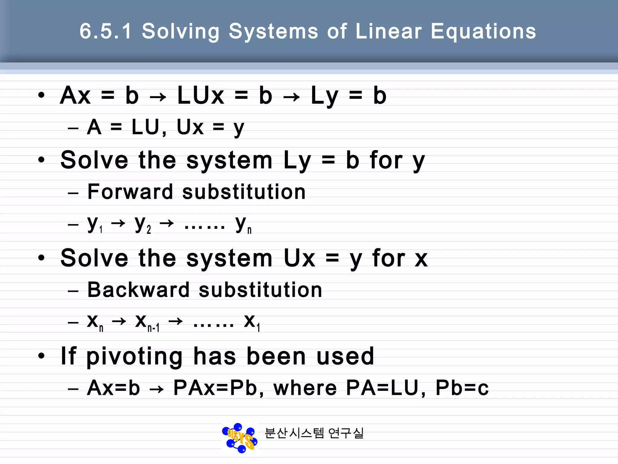
LU Factorization from Gaussian
Elimination
- MATLAB Function for LU Factorization
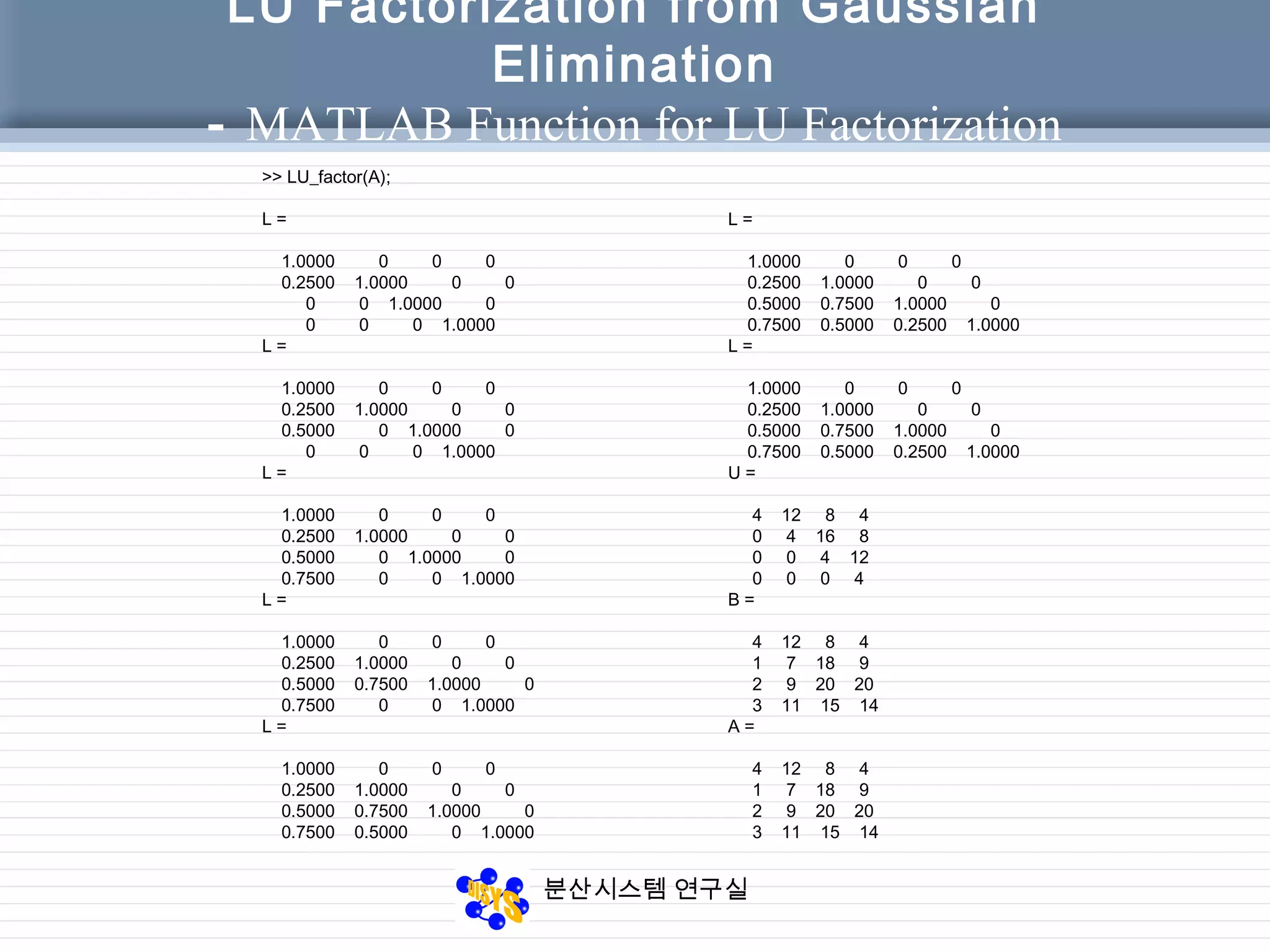
6.1.1 MATLAB Function for LU Factorization
Using Gaussian Elimination
function [L, U] = LU_Factor(A)
% LU factorization of matrix A
% using Gaussian elimination without pivoting
% Input : A n-by-n matrix
% Output L ( lower triangular ) and
% U (upper triangular )
[n, m] = size(A);
L = eye(n); % initialize matrices
U = A;
for j = 1 : n
for I = j + 1 : n
L( i , j ) = U( i, j ) / U( j, j );
U( i , : ) = U( i, j ) / L( j, j ) * U( j, : );
end
end
% display L and U
L
U
% verify results
B = L * U
A](https://image.slidesharecdn.com/chapter06-150207155631-conversion-gate02/75/Factorization-from-Gaussian-Elimination-9-2048.jpg)
![분산시스템 연구실
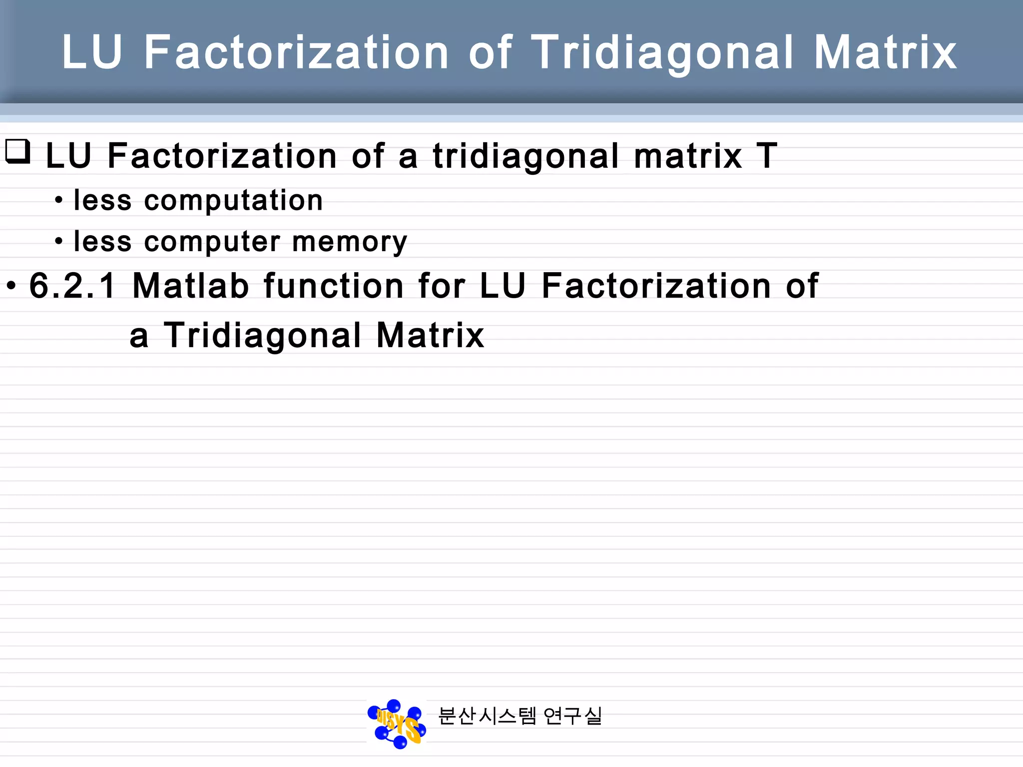
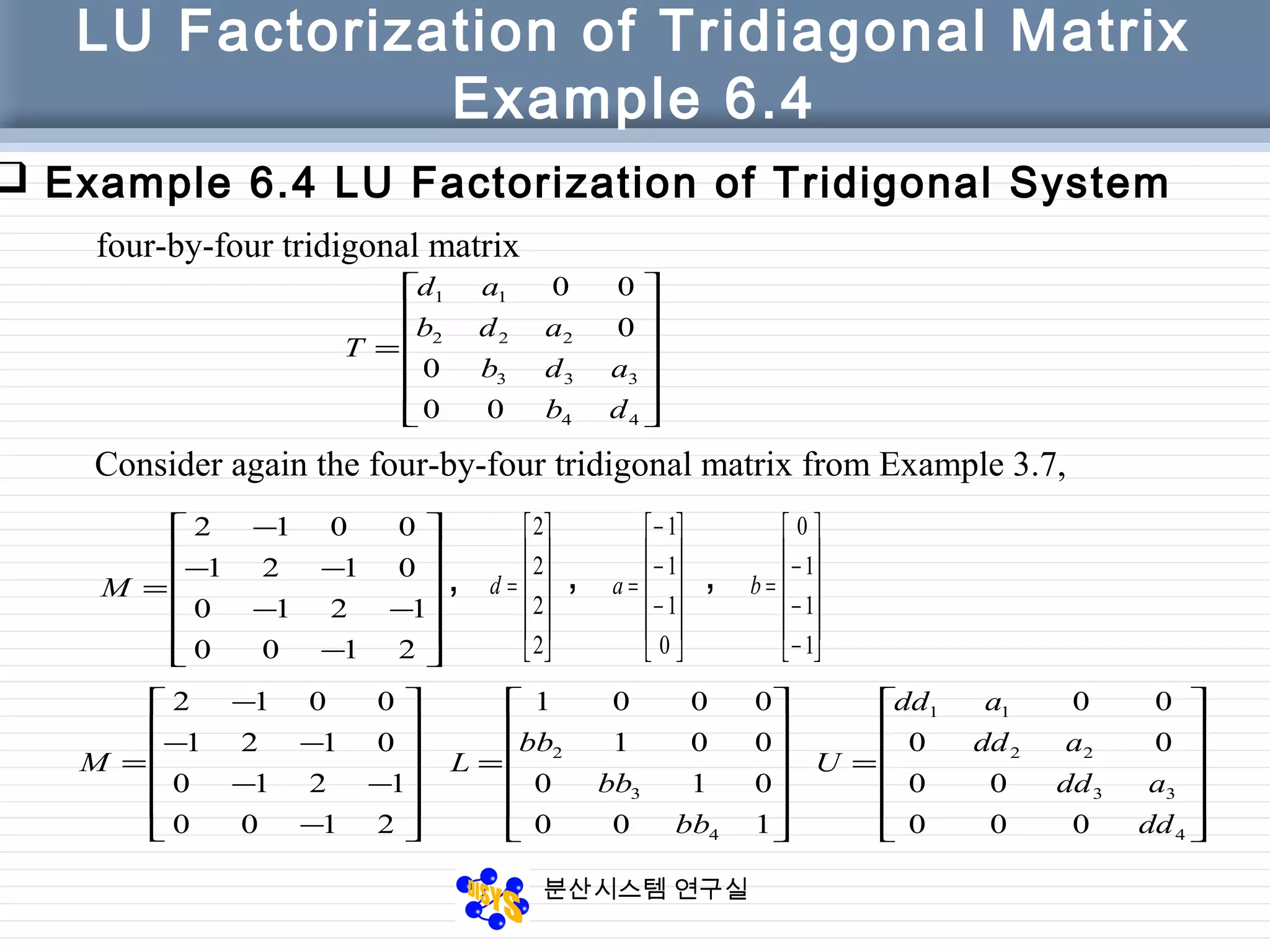
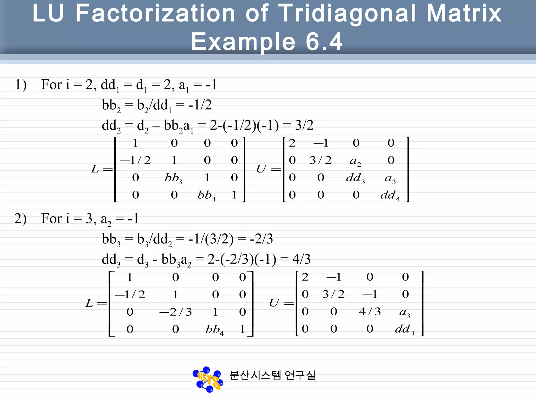
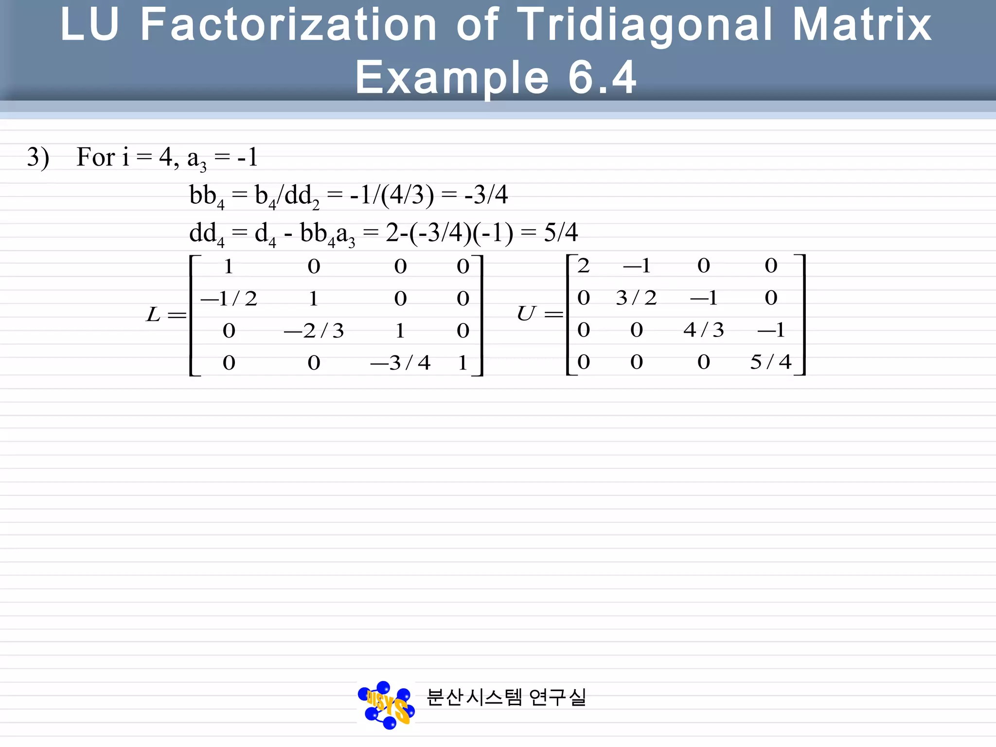
LU Factorization of Tridiagonal Matrix
function [dd, bb] = LU_tridiag(a, d, b)
% LU factorization of a tridiagonal matrix T
% Input
% a vector of elements above main diagonal, a(n) = 0
% d diagonal of matrix T
% b vector of elements below main diagonal, b(1) = 0
% The factorization of T consists of
% Lower bidiagonal matrix,
% 1’s on main diagonal; lower diagonal is bb
% Upper bidiagonal matrix,
% main diagonal is dd; upper diagonal is a
N = length(d)
bb(1) = 0;
dd(1) = d(1);
for i = 2 : n
bb(i) = b(i) / dd(i-1);
dd(i) = d(i) – bb(i) * a(i-1);
end](https://image.slidesharecdn.com/chapter06-150207155631-conversion-gate02/75/Factorization-from-Gaussian-Elimination-16-2048.jpg)

![분산시스템 연구실
6.3.5 pivoting code
Function [L, U, P] = LU_pivot(A)
[n, n1] = size(A);
L=eye(n); P=eye(n); U=A;
For j = 1:n
[pivot m] = max(abs(U(j:n, j))); m = m+j-1;
if m ~= j
% interchange rows m and j in U
% interchange rows m and j in P
if j >= 2
% interchange rows m and j in columns 1:j-1 of L
end
end
for i = j+1:n
L(i, j) = U(i, j) / U(j, j);
U(i, :) = U(i, :) – L(i, j)*U(j, :);
end
end](https://image.slidesharecdn.com/chapter06-150207155631-conversion-gate02/75/Factorization-from-Gaussian-Elimination-27-2048.jpg)

![분산시스템 연구실
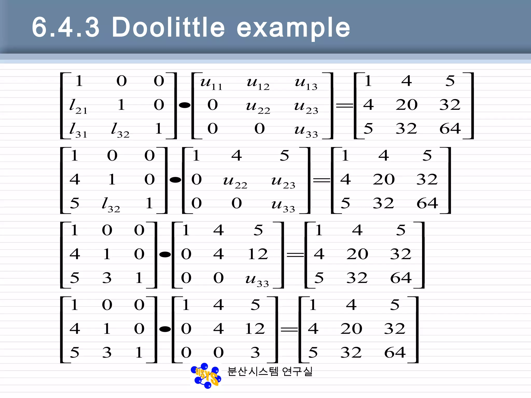
6.4.4 Doolittle code
Function [L, U] = Doolittle(A)
[n, m] = size(A);
U = zeros(n, m); L = eye(n);
for k = 1:n
U(k, k) = A(k, k) – L(k, 1:k-1)*U(1:k-1, k);
for j = k+1:n
U(k, j) = A(k, j) – L(k, 1:k-1)*U(1:k-1, j);
L(j,k)= (A(j,k)– L(j, 1:k-1)*U(1:k-1,
k))/U(k,k);
end
end](https://image.slidesharecdn.com/chapter06-150207155631-conversion-gate02/75/Factorization-from-Gaussian-Elimination-32-2048.jpg)
![분산시스템 연구실
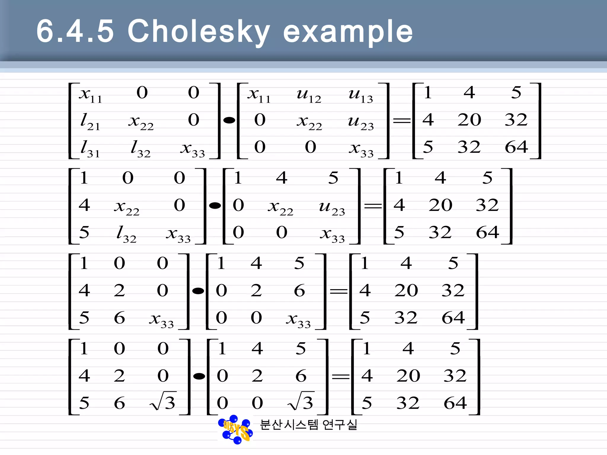
6.4.6 Cholesky code
Function [L, U] = Cholesky(A)
% A is assumed to be symmetric.
% L is computed, and U = L’
[n, m] = size(A);
L = zeros(n, n);
for k = 1:n
L(k, k) = sqrt( A(k,k) – L(k, 1:k-1)*L(k, 1:k-1)’ );
for i = k+1:n
L(i, k) = (A(i,k) – L(i, 1:k-1)*L(k, 1:k-1)’)/L(k,
k);
end
end](https://image.slidesharecdn.com/chapter06-150207155631-conversion-gate02/75/Factorization-from-Gaussian-Elimination-34-2048.jpg)
![분산시스템 연구실
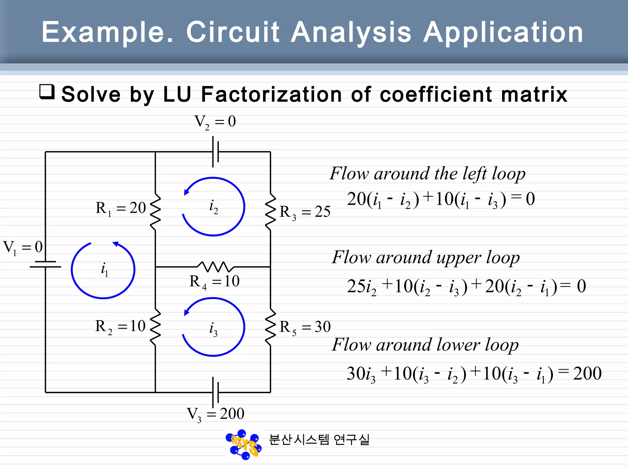
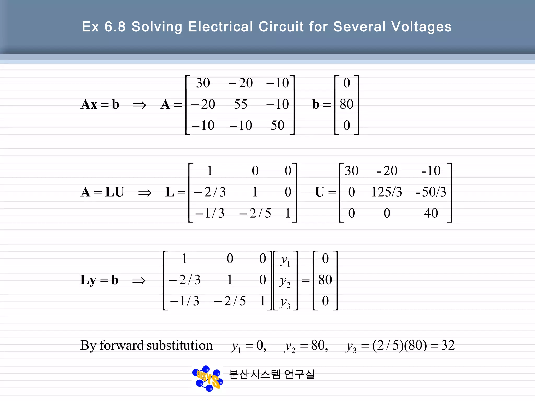
Ex 6.8 Solving Electrical Circuit for Several Voltages
11
22
33
3
2
1
0.8044/2510(4/5)]-(56/25)(1/30)[-20
2.2456/255)40/3)(3/12(80
0.804/532/40
onsubstitutibackwardBy
32
80
0
4000
3/503/1250
1020-30
ix
ix
ix
x
x
x
←===
←==+=
←===
=
−
−
⇒= yUx](https://image.slidesharecdn.com/chapter06-150207155631-conversion-gate02/75/Factorization-from-Gaussian-Elimination-39-2048.jpg)
![분산시스템 연구실
MATLAB Function to Solve the Linear System LUx=b
function x = LU_Solve(L, U, b)
% Function to solve the equation L U x = b
% L --> Lower triangular matrix (with 1's on diagonal)
% U --> Upper triangular matrix
% b --> Right-hand side vector
[n m] = size(L); z = zeros(n,1); x = zeros(n,1);
% Solve L z = b using forward substitution
z(1) = b(1);
for i = 2:n
z(i) = b(i) - L(i, 1:i-1) * z(1:i-1);
end
% Solve U x = z using back substitution
x(n) = z(n) / U(n, n);
for i = n-1 : -1 : 1
x(i) = (z(i) - U(i,i+1:n) * x(i+1:n)) / U(i, i);
end](https://image.slidesharecdn.com/chapter06-150207155631-conversion-gate02/75/Factorization-from-Gaussian-Elimination-40-2048.jpg)
![분산시스템 연구실
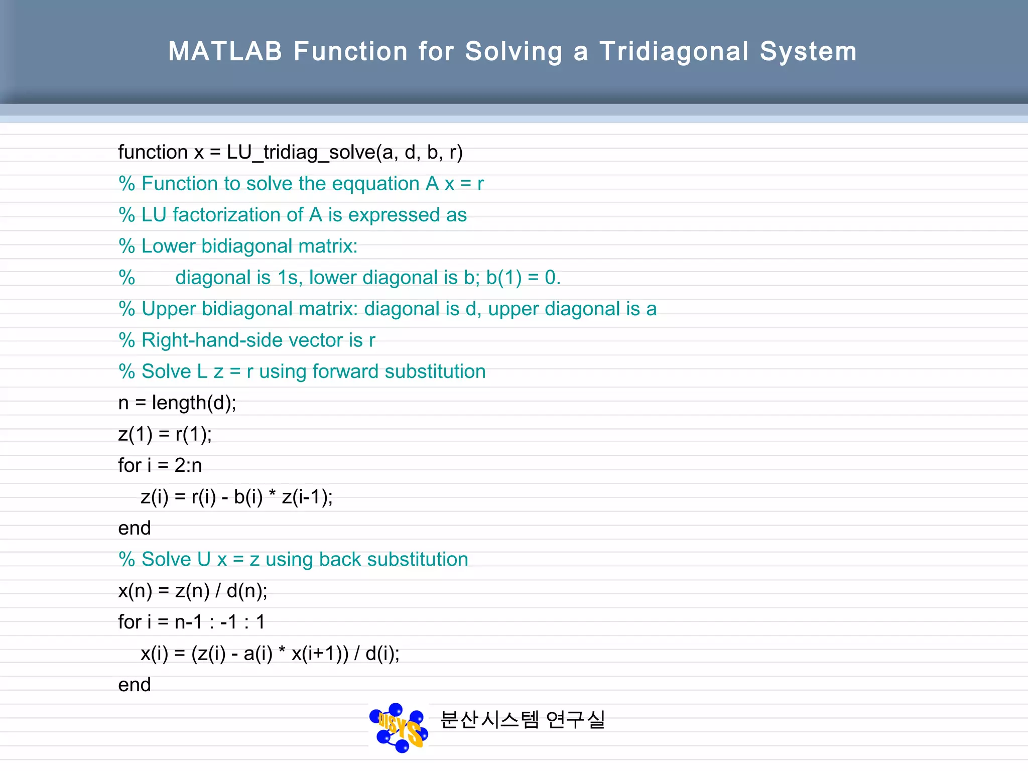
6.5.2 Solving a Tridiagonal System
[ ] [ ]
[ ]
[ ] [ ]
[ ]54-32-1
r)bb,dd,_solve(a,LU_tridiag
1111-143240
2173151
4324005214
89
6
5
23
7
214000
57300
02320
001154
00041
=
=
=−=
⇒=
==
−
−
=
−=⇒=
x
x
ddb
d
bba
rArAx
Ex 6.9](https://image.slidesharecdn.com/chapter06-150207155631-conversion-gate02/75/Factorization-from-Gaussian-Elimination-41-2048.jpg)
![분산시스템 연구실
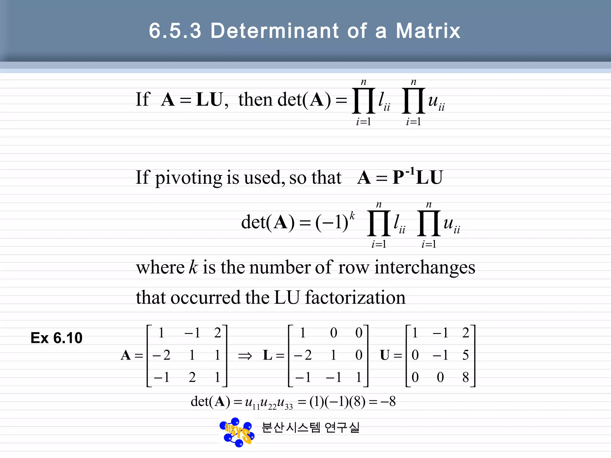
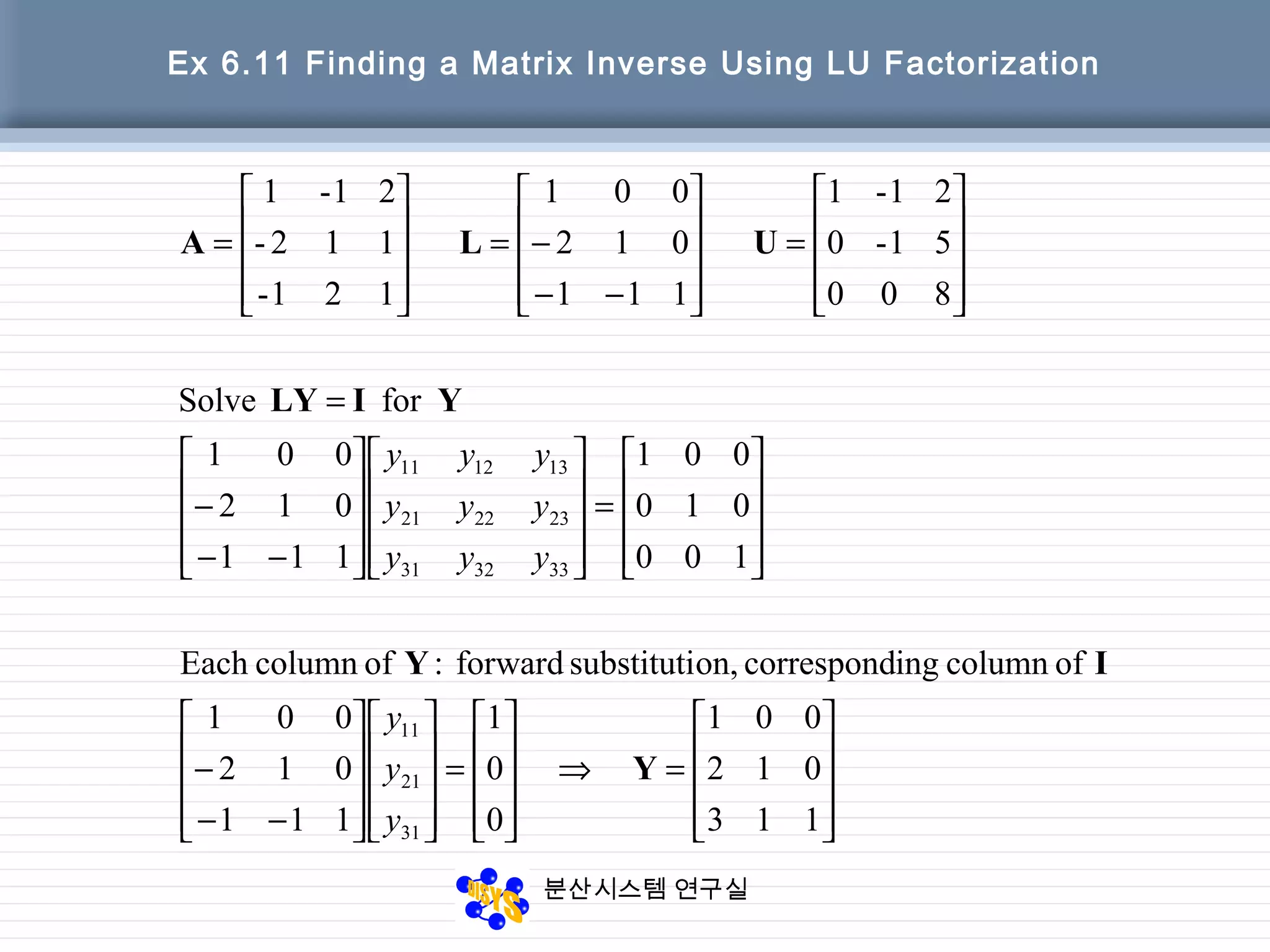
6.5.4 Inverse of a Matrix
• The inverse of an n-by-n matrix A
Axi=ei (i=1, … ,n)
– ei=[0 0 … 1 … 0 0]’, where the 1 appears
in the ith position
– X whose columns are the solution vectors
x1, … , xn is A-1](https://image.slidesharecdn.com/chapter06-150207155631-conversion-gate02/75/Factorization-from-Gaussian-Elimination-44-2048.jpg)

![분산시스템 연구실
MATLAB Function
function x = LU_Solve_Gen(L, U, B)
% Function to solve the equation L U x = B
% L --> Lower triangular matrix (1's on diagonal)
% U --> Upper triangular matrix
% B --> Right-hand-side matrix
[n n2] = size(L); [m1 m] = size(B);
% Solve L z = B using forward substitution
for j = 1:m
z(1, j) = b(1, j);
for i = 2 : n
z(i,j) = B(i,j) - L(i, 1:i-1) * z(1:i-1, j);
end
end
% Solve U x = z using back substitution
for j = 1:m
x(n, j) = z(n, j) / U(n, n);
for i = n-1 : -1 : 1
x(i,j) = (z(i,j)-U(i,i+1:n)*x(i+1:n,j)) / U(i,i);
end
end](https://image.slidesharecdn.com/chapter06-150207155631-conversion-gate02/75/Factorization-from-Gaussian-Elimination-47-2048.jpg)
![분산시스템 연구실
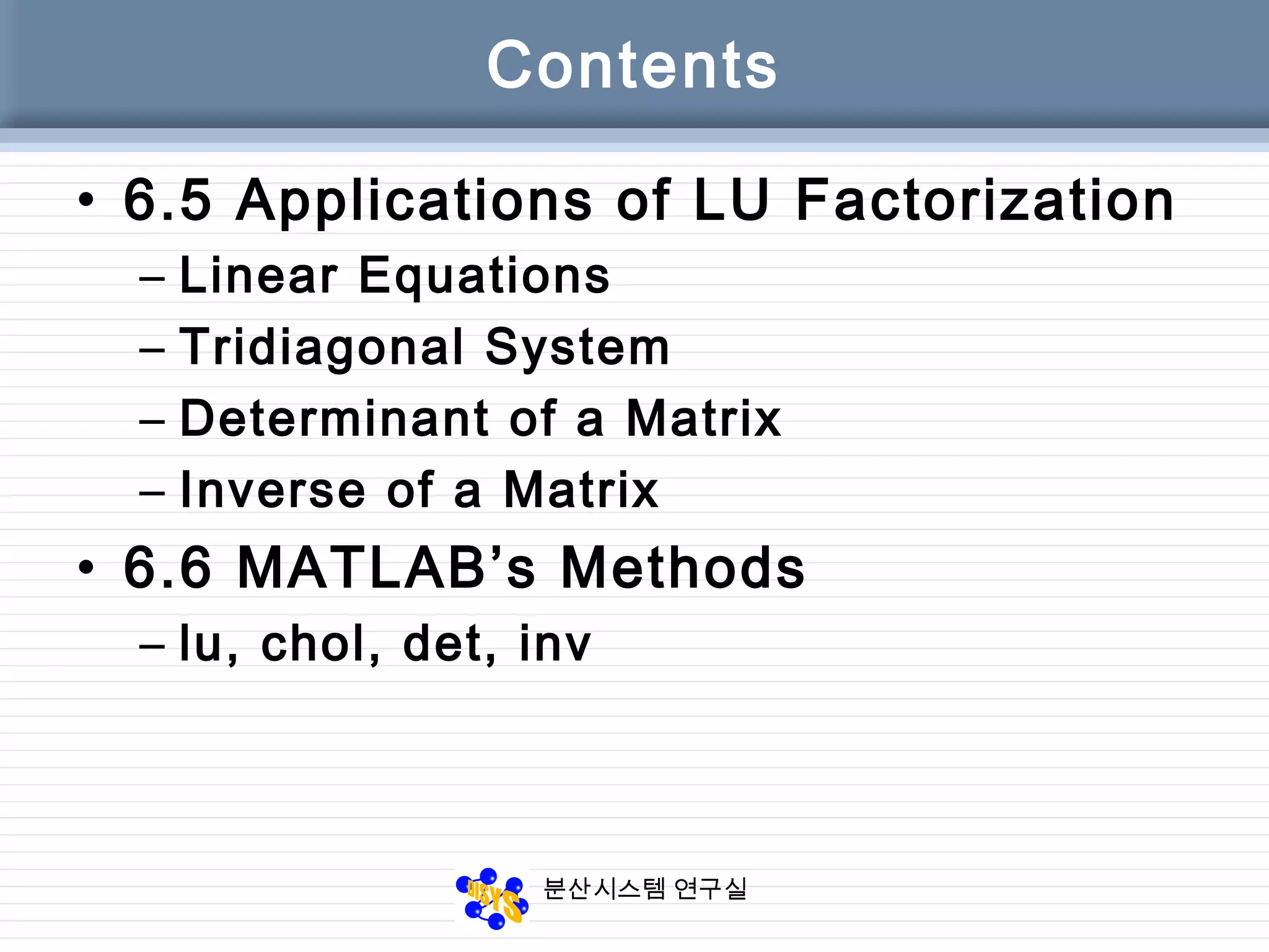
6.6 MATLAB’s Method
• 4 built-in functions
– LU decomposition of a square matrix A
• [L, U] = lu(A), [L, U, P] = lu(A)
– Cholesky factorization
• chol
– Determinant of a matrix
• det
– Inverse of a matrix
• inv](https://image.slidesharecdn.com/chapter06-150207155631-conversion-gate02/75/Factorization-from-Gaussian-Elimination-49-2048.jpg)

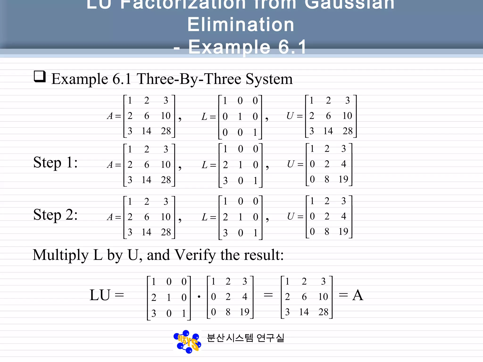
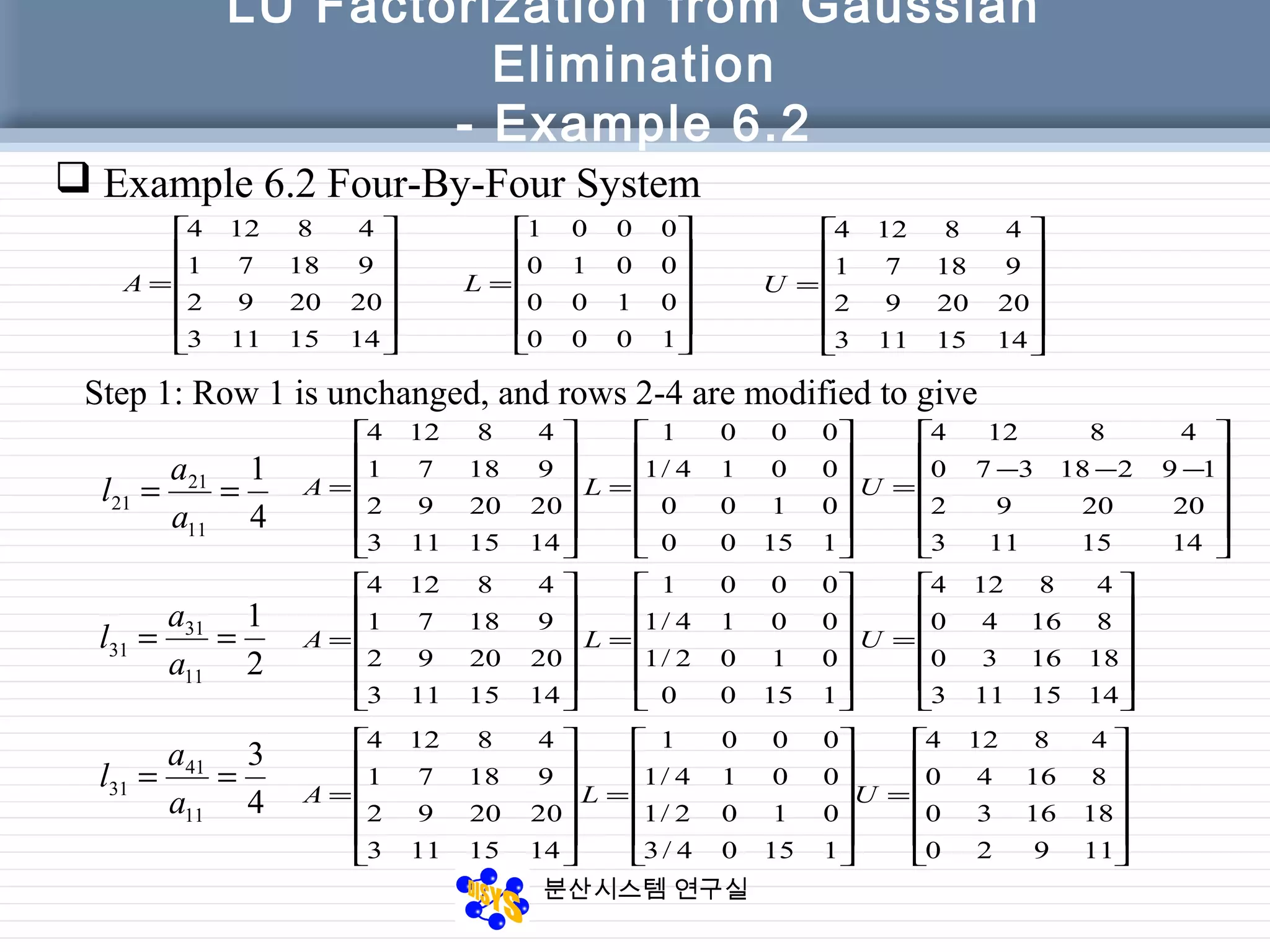
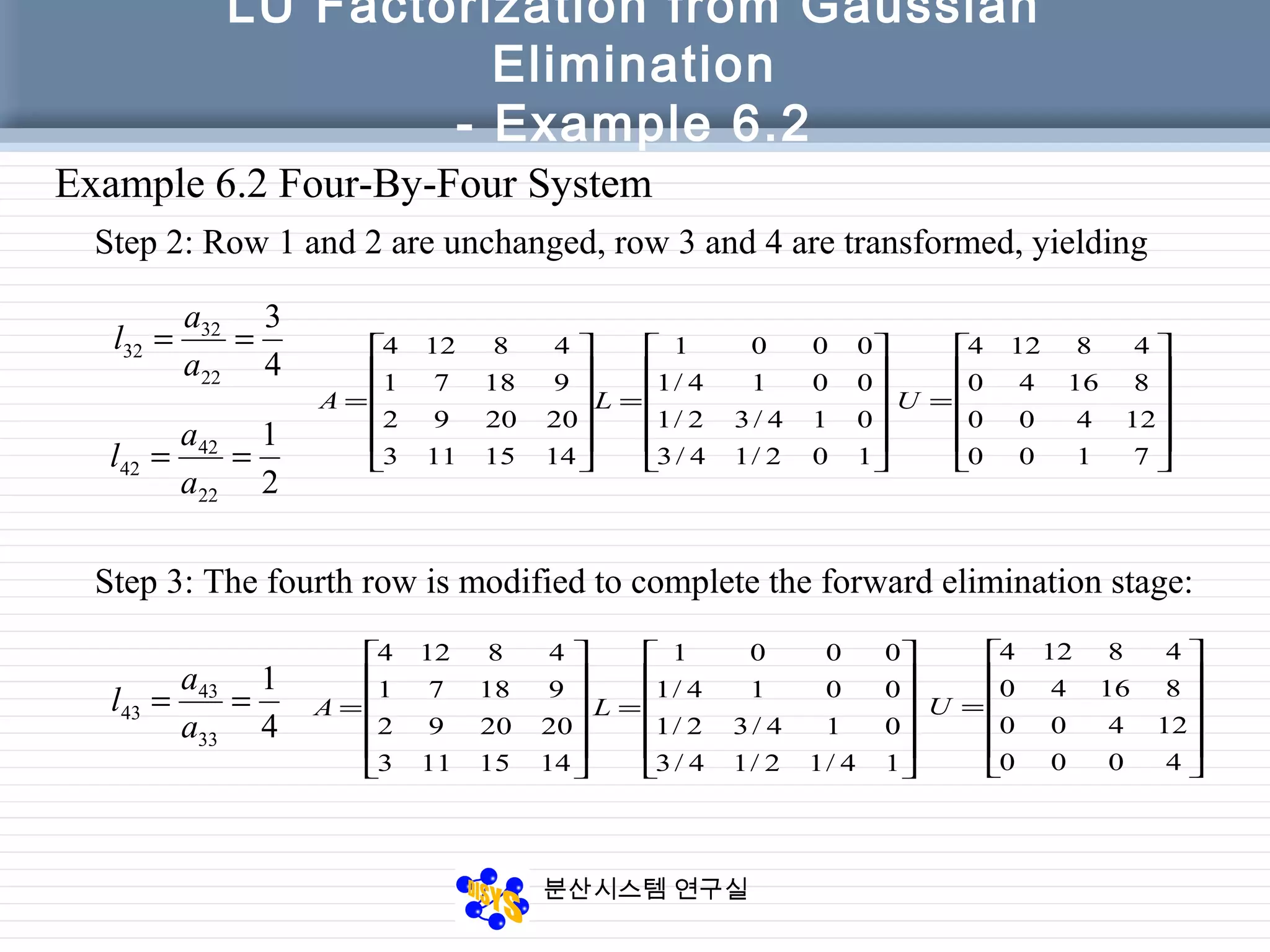
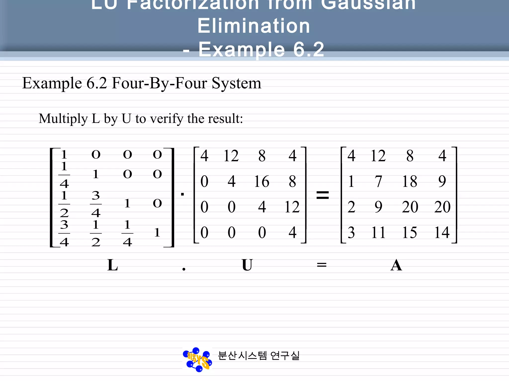
The document discusses LU factorization from Gaussian elimination. It provides examples of using Gaussian elimination to decompose matrices into lower (L) and upper (U) triangular matrices. Example 6.1 shows decomposing a 3x3 matrix, Example 6.2 a 4x4 matrix. It also provides a MATLAB function for performing LU factorization without pivoting. Example 6.3 applies LU factorization to a circuit analysis problem by decomposing the coefficient matrix.