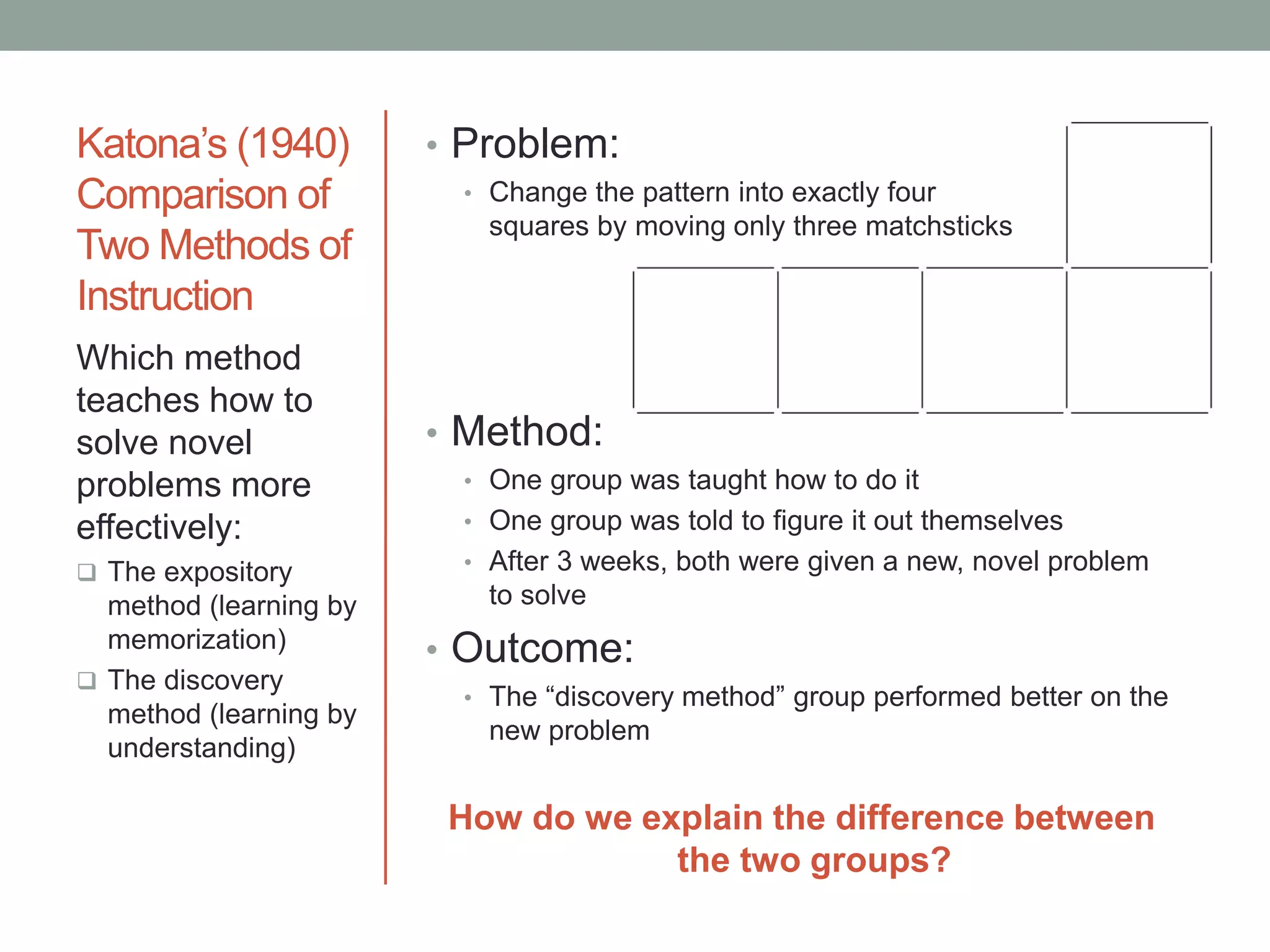
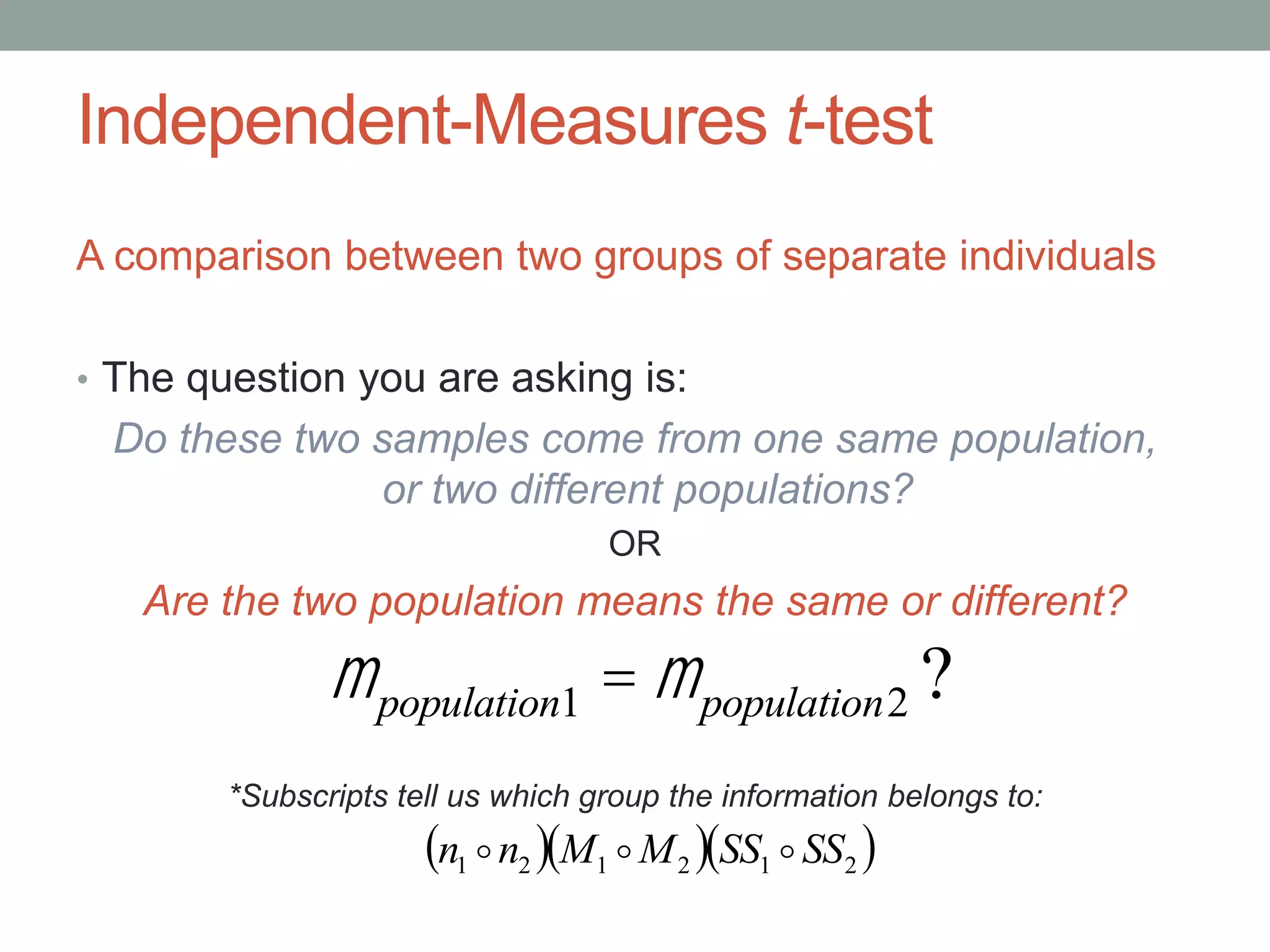
The document describes a study that compared two methods of instruction. One group was taught a problem-solving method directly, while the other group was told to figure it out themselves (the "discovery method"). After 3 weeks, both groups were given a novel problem to solve. The discovery method group performed better. The document discusses using a t-test to determine if the difference in performance was statistically significant or due to chance. It provides the formula for an independent samples t-test when comparing means between two unrelated groups. The t-test calculates whether the difference between two sample means is larger than would be expected by chance, given the variability in the samples.


![Reporting the Results
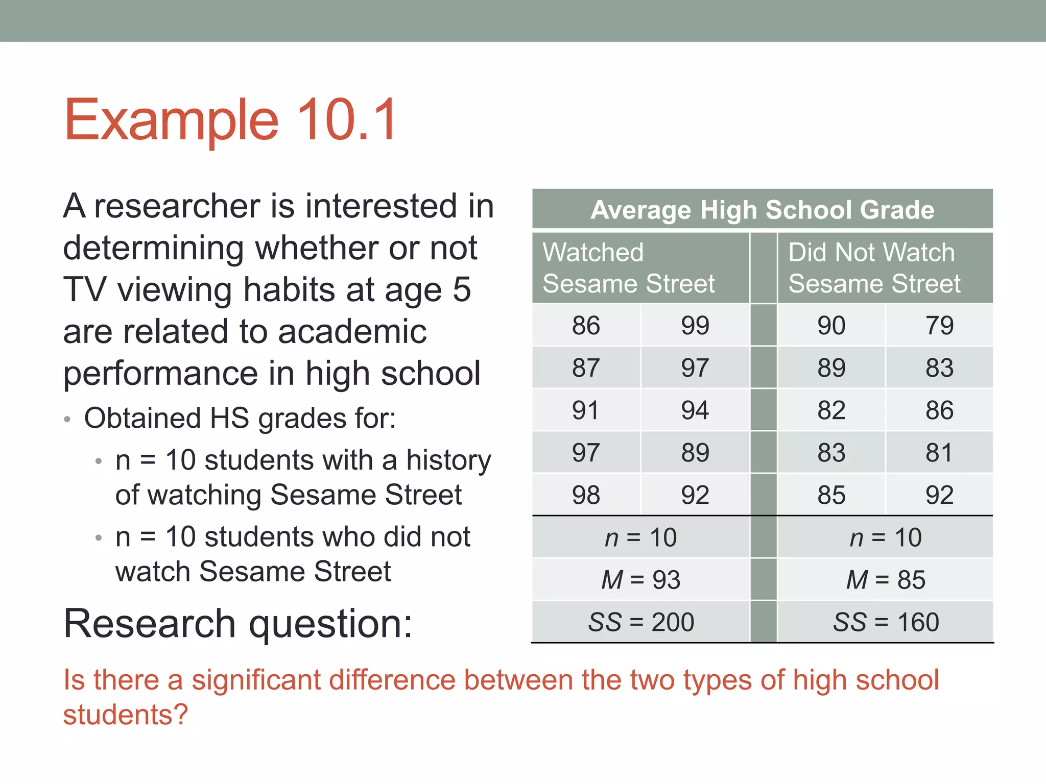
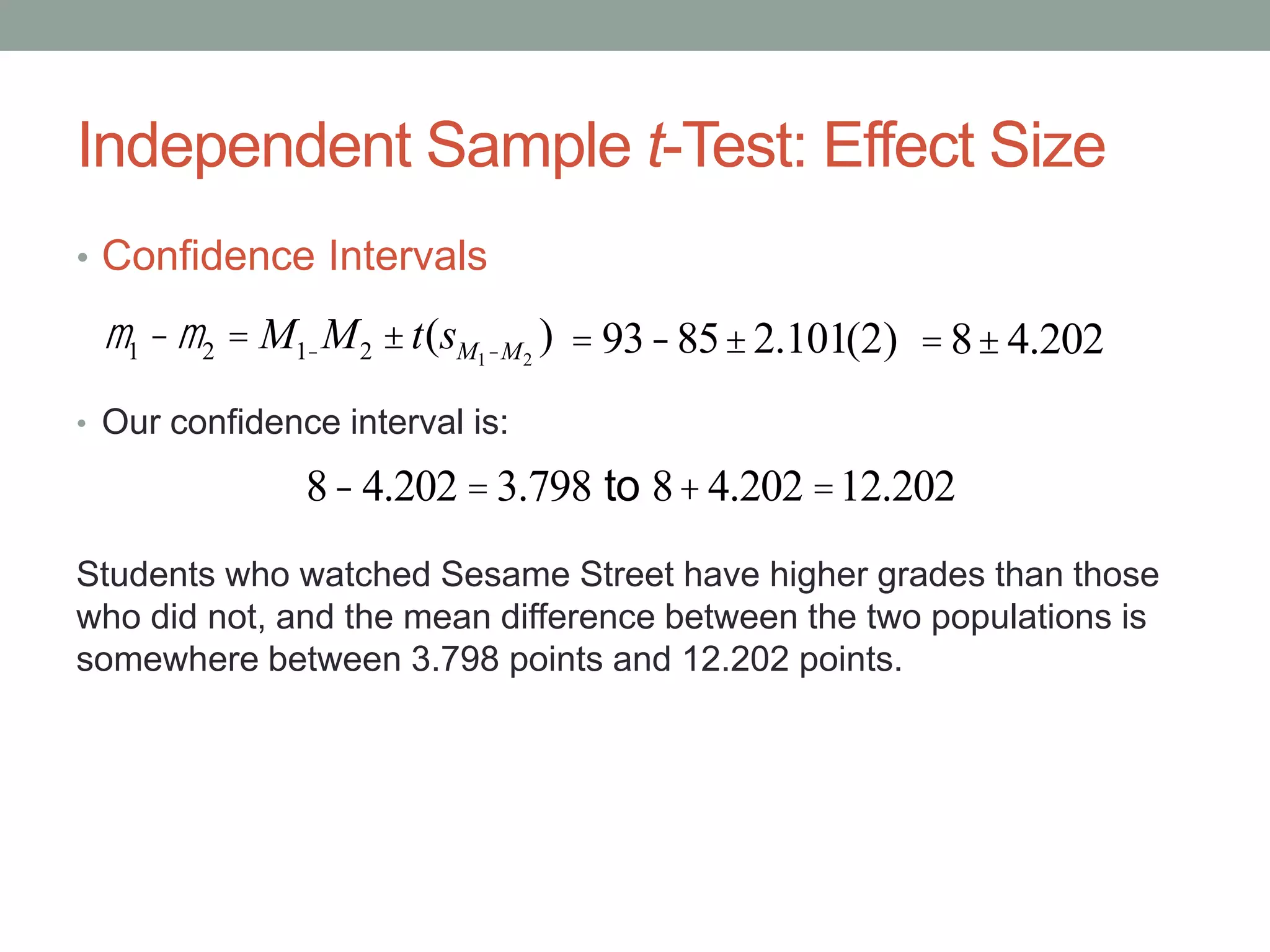
The students who watched Sesame Street as children had higher
high school grades (M = 93, SD = 4.71) than the students who did
not watch the program (M = 85, SD = 4.22). The mean difference
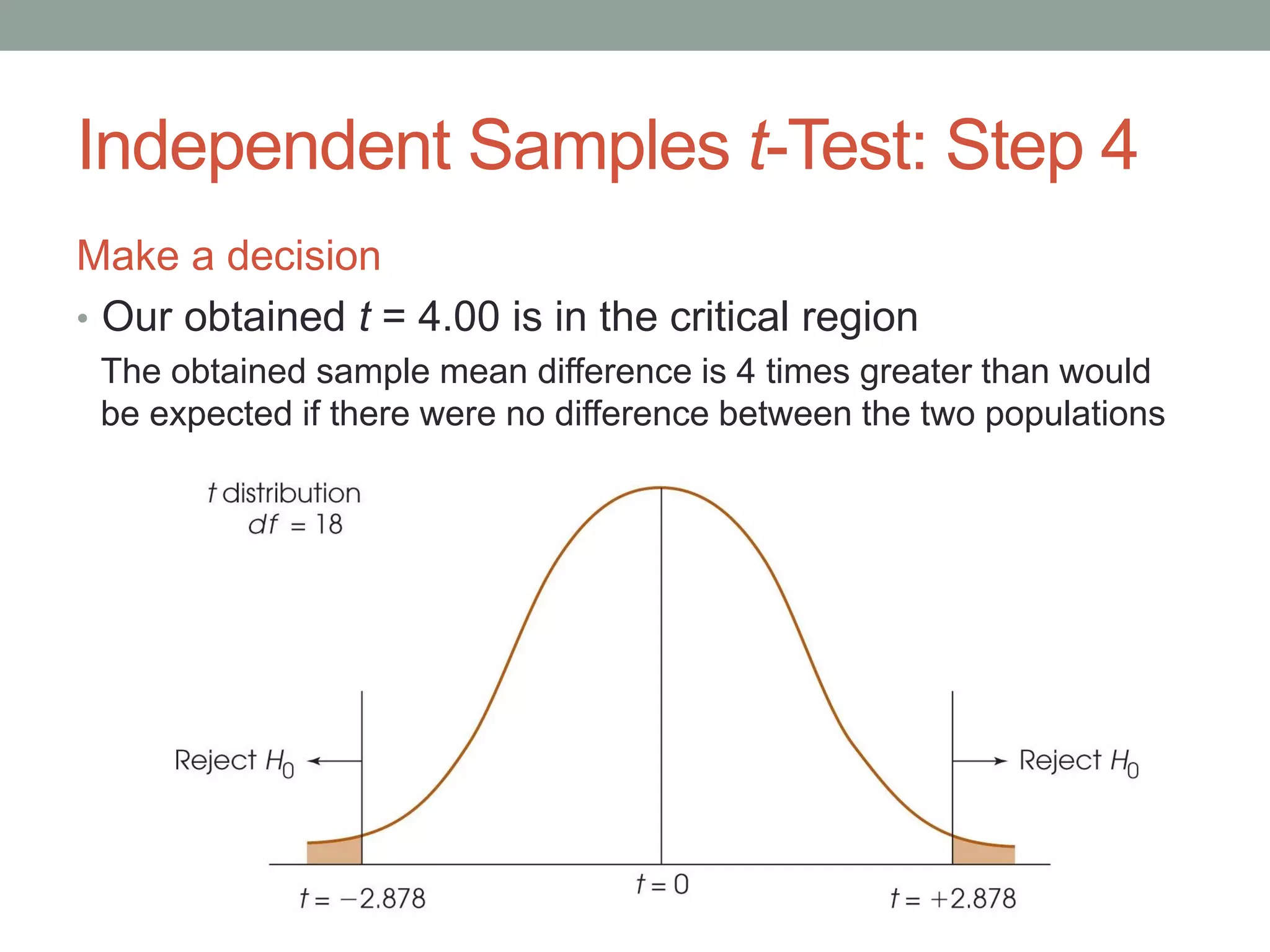
was significant, t(18) = 4.00, p < .01, d = 1.79.
• When using SPSS, you will have the exact probability (in this case
p = .001), which you would report instead of “p < .01”
t(18) = 4.00, p = .001, d = 1.79.
• If you are using confidence intervals to describe the effect size, then
you would state:
…The mean difference was significant, t(18) = 4.00, p = .001,
95% CI [3.798, 12.202]](https://image.slidesharecdn.com/chapter10indt-test-170706210305/75/Independent-samples-t-test-37-2048.jpg)