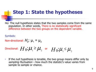
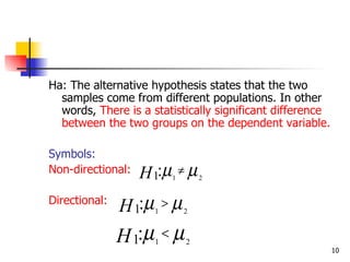
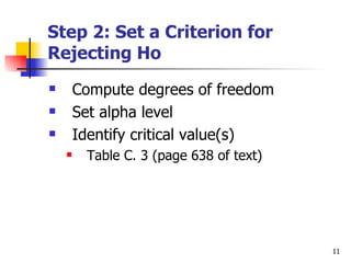
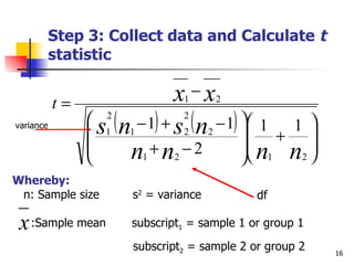
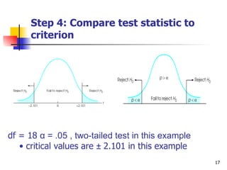
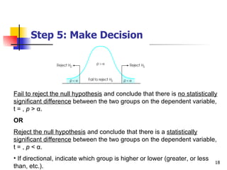
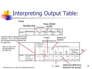
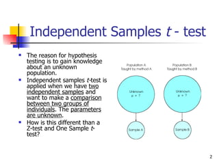
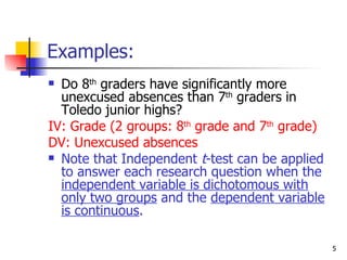
Week 9:Independent t -test


  t test for Two Independent Samples


                                       1
Independent Samples t - test
   The reason for hypothesis
    testing is to gain knowledge
    about an unknown
    population.
   Independent samples t-test is
    applied when we have two
    independent samples and
    want to make a comparison
    between two groups of
    individuals. The parameters
    are unknown.
   How is this different than a
    Z-test and One Sample t-
    test?


                                    2
Independent t - test
   We are interested in the difference between
    two independent groups. As such, we are
    comparing two populations by evaluating the
    mean difference.
   In order to evaluate the mean difference
    between two populations, we sample from
    each population and compare the sample
    means on a given variable.
   Must have two independent groups
    (i.e.samples) and one dependent variable that
    is continuous to compare them on.

                                                3
Examples:
 Do males and females significantly differ on
  their level of math anxiety?
IV: Gender (2 groups: males and females)
DV: Level of math anxiety
 Do older people exercise significantly less

  frequently than younger people?
IV: Age (2 groups: older people and younger
  people)
DV: Frequency of getting exercise

                                                 4
Examples:
 Do 8th graders have significantly more
  unexcused absences than 7th graders in
  Toledo junior highs?
IV: Grade (2 groups: 8th grade and 7th grade)
DV: Unexcused absences
 Note that Independent t-test can be applied
  to answer each research question when the
  independent variable is dichotomous with
  only two groups and the dependent variable
  is continuous.

                                                5
Generate examples of research questions
requiring an Independent Samples t-test:

   What are some examples that you can
    come up with? Remember- you need
    two independent samples and one
    dependent variable that is continuous.


                                             6
Assumptions
   The two groups are independent of one another.

   The dependent variable is normally distributed.
       Examine skewness and kurtosis (peak) of distribution
            Leptokurtosis vs. platykurtosis vs. mesokurtosis


   The two groups have approximately equal
    variance on the dependent variable. (When n1 = n2
    [equal sample sizes] ,the violation of this
    assumption has been shown to be unimportant.)

                                                                7
Steps in Independent Samples t-test


                                      8
Step 1: State the hypotheses

Ho: The null hypothesis states that the two samples come from the same
  population. In other words, There is no statistically significant
  difference between the two groups on the dependent variable.

Symbols:
Non-directional:   Ho: μ1 = μ2

Directional:   H 0:µ ≥ µ1      2
                                   or
                                        H 0:µ ≤ µ 1      2


•   If the null hypothesis is tenable, the two group means differ only by
    sampling fluctuation – how much the statistic’s value varies from
    sample to sample or chance.
                                                                            9
Ha: The alternative hypothesis states that the two
  samples come from different populations. In other
  words, There is a statistically significant difference
  between the two groups on the dependent variable.

Symbols:
Non-directional:   H 1:µ ≠ µ
                         1       2


Directional:
               H 1:µ > µ
                     1       2


               H 1:µ < µ
                     1       2
                                                           10
Step 2: Set a Criterion for
Rejecting Ho
       Compute degrees of freedom
       Set alpha level
       Identify critical value(s)
        Table C. 3 (page 638 of text)


                                         11
Computing Degrees of Freedom
Calculate degrees of freedom (df) to determine
 rejection region.
         n n
df = 1 + 2 − 2
                                           -2
    sample size for sample1+ sample size for sample2
    •   df describe the number of scores in a sample that are
        free to vary.
    •   We subtract 2 because in this case we have 2
        samples.


                                                            12
More on Degrees of Freedom

•   In an Independent samples t-test, each
    sample mean places a restriction on the
    value of one score in the sample, hence
    the sample lost one degree of freedom and
    there are n-1 degrees of freedom for the
    sample.


                                            13
Set alpha level
   Set at .001, .01 , .05, or .10, etc.


                                           14
Identify critical value(s)
   Directional or non-directional?
   Look at page 638 Table C.3.
   To determine your CV(s) you need to
    know:
       df – if df are not in the table, use the next
        lowest number to be conservative
       directionality of the test
       alpha level

                                                        15
Step 3: Collect data and Calculate t
           statistic


           t=             x −x    1       2

                 ( − 1) + ( − 1)  1
                  2               2
                                                        
variance
                s n
                  1   1   s n  + 1
                                  2   2                 
                    n +n −2       n n                
                         1   2                  1   2

Whereby:
 n: Sample size       s2 = variance           df

 x :Sample mean       subscript1 = sample 1 or group 1
                      subscript2 = sample 2 or group 2      16
Step 4: Compare test statistic to
      criterion


df = 18 α = .05 , two-tailed test in this example
   • critical values are ± 2.101 in this example
                                                    17
Step 5: Make Decision


Fail to reject the null hypothesis and conclude that there is no statistically
significant difference between the two groups on the dependent variable,
t = , p > α.
OR
Reject the null hypothesis and conclude that there is a statistically
significant difference between the two groups on the dependent variable,
t = , p < α.
• If directional, indicate which group is higher or lower (greater, or less
                                                                              18
than, etc.).
Interpreting Output Table:
                                                          Mean APGAR
                                    Sample size             SCORE


Levene’s tests the assumption of equal
variances – if p < .05, then variances
                                                          t-value        Degrees of
are not equal and use a different test                                   freedom
to modify this:

  Here, we have met
  the assumption so
  use first row.                                                                                      CI


                                                                    p - value
                                                                                Observed difference        19
   Retrieved on July 12, 2007 from SPSSShortManual.html                         between the groups
Interpreting APA table:


                          20
Variable                       Math anxiety   t
 Gender
  Male                             3.66
  Female                           3.98        3.35***
 Age
  Under 40 years                   3.32
  Over 41 years                    3.64        2.67**
Note. **p < .01. ***p < .001.
                                                         21
Examples and Practice
   See attached document.
   Create the following index cards from this
    lecture:
       When to conduct a t-test (purpose, conditions,
        and assumptions)
       t-test statistic formula for computation
            t-test statistic formula
            df formula


                                                         22

T Test For Two Independent Samples

  • 1.
    Week 9:Independent t-test t test for Two Independent Samples 1
  • 2.
    Independent Samples t- test  The reason for hypothesis testing is to gain knowledge about an unknown population.  Independent samples t-test is applied when we have two independent samples and want to make a comparison between two groups of individuals. The parameters are unknown.  How is this different than a Z-test and One Sample t- test? 2
  • 3.
    Independent t -test  We are interested in the difference between two independent groups. As such, we are comparing two populations by evaluating the mean difference.  In order to evaluate the mean difference between two populations, we sample from each population and compare the sample means on a given variable.  Must have two independent groups (i.e.samples) and one dependent variable that is continuous to compare them on. 3
  • 4.
    Examples:  Do malesand females significantly differ on their level of math anxiety? IV: Gender (2 groups: males and females) DV: Level of math anxiety  Do older people exercise significantly less frequently than younger people? IV: Age (2 groups: older people and younger people) DV: Frequency of getting exercise 4
  • 5.
    Examples:  Do 8thgraders have significantly more unexcused absences than 7th graders in Toledo junior highs? IV: Grade (2 groups: 8th grade and 7th grade) DV: Unexcused absences  Note that Independent t-test can be applied to answer each research question when the independent variable is dichotomous with only two groups and the dependent variable is continuous. 5
  • 6.
    Generate examples ofresearch questions requiring an Independent Samples t-test:  What are some examples that you can come up with? Remember- you need two independent samples and one dependent variable that is continuous. 6
  • 7.
    Assumptions  The two groups are independent of one another.  The dependent variable is normally distributed.  Examine skewness and kurtosis (peak) of distribution  Leptokurtosis vs. platykurtosis vs. mesokurtosis  The two groups have approximately equal variance on the dependent variable. (When n1 = n2 [equal sample sizes] ,the violation of this assumption has been shown to be unimportant.) 7
  • 8.
    Steps in IndependentSamples t-test 8
  • 9.
    Step 1: Statethe hypotheses Ho: The null hypothesis states that the two samples come from the same population. In other words, There is no statistically significant difference between the two groups on the dependent variable. Symbols: Non-directional: Ho: μ1 = μ2 Directional: H 0:µ ≥ µ1 2 or H 0:µ ≤ µ 1 2 • If the null hypothesis is tenable, the two group means differ only by sampling fluctuation – how much the statistic’s value varies from sample to sample or chance. 9
  • 10.
    Ha: The alternativehypothesis states that the two samples come from different populations. In other words, There is a statistically significant difference between the two groups on the dependent variable. Symbols: Non-directional: H 1:µ ≠ µ 1 2 Directional: H 1:µ > µ 1 2 H 1:µ < µ 1 2 10
  • 11.
    Step 2: Seta Criterion for Rejecting Ho  Compute degrees of freedom  Set alpha level  Identify critical value(s)  Table C. 3 (page 638 of text) 11
  • 12.
    Computing Degrees ofFreedom Calculate degrees of freedom (df) to determine rejection region. n n df = 1 + 2 − 2 -2 sample size for sample1+ sample size for sample2 • df describe the number of scores in a sample that are free to vary. • We subtract 2 because in this case we have 2 samples. 12
  • 13.
    More on Degreesof Freedom • In an Independent samples t-test, each sample mean places a restriction on the value of one score in the sample, hence the sample lost one degree of freedom and there are n-1 degrees of freedom for the sample. 13
  • 14.
    Set alpha level  Set at .001, .01 , .05, or .10, etc. 14
  • 15.
    Identify critical value(s)  Directional or non-directional?  Look at page 638 Table C.3.  To determine your CV(s) you need to know:  df – if df are not in the table, use the next lowest number to be conservative  directionality of the test  alpha level 15
  • 16.
    Step 3: Collectdata and Calculate t statistic t= x −x 1 2  ( − 1) + ( − 1)  1 2 2  variance s n 1 1 s n  + 1 2 2   n +n −2  n n   1 2  1 2 Whereby: n: Sample size s2 = variance df x :Sample mean subscript1 = sample 1 or group 1 subscript2 = sample 2 or group 2 16
  • 17.
    Step 4: Comparetest statistic to criterion df = 18 α = .05 , two-tailed test in this example • critical values are ± 2.101 in this example 17
  • 18.
    Step 5: MakeDecision Fail to reject the null hypothesis and conclude that there is no statistically significant difference between the two groups on the dependent variable, t = , p > α. OR Reject the null hypothesis and conclude that there is a statistically significant difference between the two groups on the dependent variable, t = , p < α. • If directional, indicate which group is higher or lower (greater, or less 18 than, etc.).
  • 19.
    Interpreting Output Table: Mean APGAR Sample size SCORE Levene’s tests the assumption of equal variances – if p < .05, then variances t-value Degrees of are not equal and use a different test freedom to modify this: Here, we have met the assumption so use first row. CI p - value Observed difference 19 Retrieved on July 12, 2007 from SPSSShortManual.html between the groups
  • 20.
  • 21.
    Variable Math anxiety t Gender Male 3.66 Female 3.98 3.35*** Age Under 40 years 3.32 Over 41 years 3.64 2.67** Note. **p < .01. ***p < .001. 21
  • 22.
    Examples and Practice  See attached document.  Create the following index cards from this lecture:  When to conduct a t-test (purpose, conditions, and assumptions)  t-test statistic formula for computation  t-test statistic formula  df formula 22