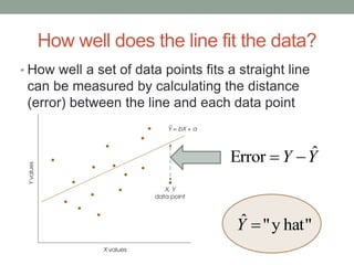
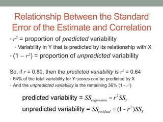
CHAPTER 16
Regression
Regression
The statistical technique for finding the best-fitting straight
line for a set of data
• Allows us to make
predictions based on
correlations
• A linear relationship
between two variables
allows the computation
of an equation that
provides a precise,
mathematical description
of the relationship abXY 
Regression
Line
The Relationship Between
Correlation and Regression
Both examine the relationship/association
between two variables
Both involve an X and Y variable for each
individual (one pair of scores)
Differences in practice
Correlation
Used to determine the
relationship between
two variables
Regression
Used to make
predictions about one
variable based on the
value of another
The Linear Equation:
Expresses a linear relationship between variables X and Y
• X: represents any given score on X
• Y: represents the corresponding score for Y based on X
• a: the Y-intercept
• Determines what the
value of Y equals when X = 0
• Where the line crosses the
Y-axis
• b: the slope constant
• How much the Y variable
will change when X is
increased by one point
• The direction and degree of the line’s tilt
abXY 
Prediction using Regression
A local video store charges a
$5/month membership fee
which allows video rentals at
$2 each
• How much will I spend per
month?
• If you never rent a video (X = 0)
• If you rent 3 videos/mo (X = 3)
• If you rent 8 videos/mo (X = 8)
abXY 
52  XY
55)0(2 Y
115)3(2 Y
215)8(2 Y
Graphing linear equations
7560)35(3
6060)05(0


YX
YX
The intercept (a) is 60
(when X = 0, Y = 60)
The slope (b) is 5
(as we increase one value in X, Y
increases 5 points)
0
10
20
30
40
50
60
70
80
0 1 2 3 4
• To graph the line below,
we only need to find two
pairs of scores for X and Y,
and then draw the straight
line that connects them
605  XY
The Regression Line
The line through the data points that ‘best fit’ the data
(assuming a linear relationship)
1. Makes the relationship
between two variables
easier to see (and
describe)
2. Identifies the ‘central
tendency’ of the relationship
between the variables
3. Can be used for prediction
• Best fit: the line that minimizes the distance of each
point to the line
‘Best fit’
Regression
Line
Correlation and the regression line
0
1
2
3
4
5
6
7
8
0 1 2 3 4 5
• The magnitude of the
correlation coefficient (r ) is
an indicator of how well
the points aggregate
around the regression line
• What would a perfect
correlation look like?
The Distance Between a Point and the Line
:ˆ
:
Y
Y
Each data point will have its
own distance from the
regression line (a.k.a. error)
The actual value of Y shown in
the data for a given X
The value of Y predicted for a
given X from your linear
equation
YY ˆDistance 
How well does the line fit the data?
• How well a set of data points fits a straight line
can be measured by calculating the distance
(error) between the line and each data point
YY ˆError 
hat"y"ˆ Y
How well does the line fit the data?
• Some of distances will be positive and some
negative, so to find a total value we must square
each distance (remember SS)
 2
ˆ YY
Total squared error
(SS residual):
Remember, this is
the squared sum
of all distances
The Regression Line
The line through the data points that ‘best fit’ the data
(assuming a linear relationship)
The Least-
Squared-Error
Solution
A.k.a.
• The “best fit”
regression line
• minimizes the distance
of each point from the line
• Gives the best prediction
of Y
• The Least-Squared-Error
Solution
• Results in the smallest possible
value for the total squared error abXY ˆ
Solving the regression equation
abXY ˆ
Remember:
n
YX
XYSP


x
y
x s
s
r
SS
SP
b 
XY bMMa 
meanM
I interrupt our regularly scheduled
program for a brief announcement….
‘Memba these?
We have spent the semester
utilizing the Computational
Formulas for all Sum of Squares
For sanity’s sake, we will now be
utilizing the definitional formulas
for all
n
X
XSSX
2
2 )(

n
Y
YSSY
2
2 )(

n
YX
XYSP


2
)( XX MXSS 
  YX MYMXSP 
2
)( YY MYSS 
And now back to our regularly
scheduled programming…..
Solving the regression equation
abXY ˆ
Remember:
x
y
x s
s
r
SS
SP
b 
XY bMMa 
meanM
  YX MYMXSP 
Let’s Try One!
(Example 16.1, p.563, using the definitional formula)
Scores
X Y
2 3
6 11
0 6
4 6
7 12
5 7
5 10
3 9
∑X=32
Mx=4
∑Y=64
MY=8
Error
X - MX Y - MY
-2 -5
2 3
-4 -2
0 -2
3 4
1 -1
1 2
-1 1
Products
(X – MX)(Y – MY)
10
6
8
0
12
-1
2
-1
SP = 36
Squared Error
(X - MX)2 (Y - MY)2
4 25
4 9
16 4
0 4
9 16
1 1
1 4
1 1
SSX = 36 SSY = 64
Find b and a in the regression equation
1
36
36

xSS
SP
b
448)4(18 

a
bMMa XY
36
648;364


SP
SSMSSM YYXx
441ˆ  XXabXY
Making Predictions
We use the regression to make predictions.
• For the previous example:
• Thus, an individual with a score of X = 3 would be
predicted to have a Y score of:
However, keep in mind:
1. The predicted value will not be perfect unless the correlation is
perfect (the data points are not perfectly in line)
• Least error is NOT the absence of error
2. The regression equation should not be used to make predictions for
X values outside the range of the original data
4ˆ  XY
743ˆ Y
Standardizing the Regression Equation
The standardized form of the regression equation
utilizes z-scores (standardized scores) in place of raw
scores:
Note:
1. We are now using the z-score for each X value (zx) to predict the
z-score for the corresponding Y value (zy)
2. The slope constant that was b is now identified as β (“beta”)
• The slope for standardized variables: one standard deviation change
in X produces this much change in the standard deviation of Y
• For an equation with two variables, β = Pearson r
3. There is no longer a constant (a) in the equation
because z-scores have a mean of 0
xy zz ˆ
xy bMMa 
The Accuracy of the Predictions
• These plots of two different sets of data have the same
regression equation
The regression equation does not
provide any information about the
accuracy of the predictions!
The Standard Error of the Estimate
Provides a measure of the standard distance between a
regression line (the predicted Y values) and the actual data
points (the actual Y values)
• Very similar to the standard deviation
• Answers the question:
How accurately does the regression equation predict the
observed Y values?
 
2
ˆ 2
.



n
YY
df
SS
s residual
XY
Let’s Compute the Standard Error of
Estimate (Example 16.1, p.563, using the definitional formula)
Data
X Y
2 3
6 11
0 6
4 6
5 7
7 12
5 10
3 9
Predicted Y
values
6
10
4
8
9
11
9
7
4ˆ  XY
Residual
-3
1
2
-2
-2
1
1
2
0
YY ˆ
Squared
Residual
9
1
4
4
4
1
1
4
SSresidual = 28
 2
ˆYY 
 
2
ˆ 2
.



n
YY
df
SS
s residual
XY
43.11
67.130
6
784
28
282





Relationship Between the Standard
Error of the Estimate and Correlation
• r2 = proportion of predicted variability
• Variability in Y that is predicted by its relationship with X
• (1 – r2) = proportion of unpredicted variability
So, if r = 0.80, then the predicted variability is r2 = 0.64
• 64% of the total variability for Y scores can be predicted by X
• And the unpredicted variability is the remaining 36% (1 - r2)
predicted variability = SSregression = r2
SSY
unpredicted variability = SSresidual = (1-r2
)SSY
An Easier Way to Compute SSresidual
sY.X =
SSresidual
df
=
1-r2
( )SSY
n-2
 
2
ˆ 2
.



n
YY
df
SS
s residual
XY
Instead of computing individual error values:
It is easier to simply use the formula for unpredicted
variability for the SSresidual
These are the steps we just went through to
compute the Standard Error of Estimate
Data
X Y
2 3
6 11
0 6
4 6
5 7
7 12
5 10
3 9
Predicted Y
values
6
10
4
8
9
11
9
7
4ˆ  XY
Residual
-3
1
2
-2
-2
1
1
2
0
YY ˆ
Squared
Residual
9
1
4
4
4
1
1
4
SSresidual = 28
 2
ˆYY 
sY.X =
SSresidual
df
=
å Y - ˆY( )
2
n-2
43.11
67.130
6
784
28
282





Now let’s do it using the easier formula
• We know SSX = 36, SSY = 64, and SP = 36 because we
calculated it a few slides back:
Scores
X Y
2 3
6 11
0 6
4 6
5 7
7 12
5 10
3 9
∑X=32
Mx=4
∑Y=64
MY=8
Error
X - MX Y - MY
-2 -5
2 3
-4 -2
0 -2
3 4
1 -1
1 2
-1 1
Products
(X - MX)2(Y - MY)2
10
6
8
0
12
-1
2
-1
SP = 36
Squared Error
(X - MX)2 (Y - MY)2
4 25
4 9
16 4
0 4
9 16
1 1
1 4
1 1
SSX = 36 SSY = 64
Using those figures, we can compute:
• With SSY = 64 and a correlation of 0.75, the predicted
variability from the regression equation is:
r =
SP
SSXSSY
=
36
36(64)
=
36
2304
=
36
48
= 0.75
SSregression = r2
SSY = 0.752
(64)= 0.5625(64) = 36
SSresidual = (1-r2
)SSY = (1-0.752
)64 = (1-0.5625)64
= (0.4375)64 = 28
• And the unpredicted variability is:
• This is the same value we found working with our table!
CHAPTER 16.2
Analysis of Regression:
Testing the Significance of the Regression Equation
Analysis of Regression
• Uses an F-ratio to determine whether the variance
predicted by the regression equation is significantly
greater than would be expected if there was no
relationship between X and Y.
F =
variance in Y predicted by the regression equation
unpredicted variance in the Y scores
F =
systematic changes in Y resulting from changes in X
changes in Y that are independent from changes in X
Significance testing
The regression equation does not account for a
significant proportion of variance in the Y scores
The equation does account for a significant
proportion of variance in the Y scores
MSregression =
SSregression
dfregression
;df =1
MSresidual =
SSresidual
dfresidual
;df = n- 2
Find and evaluate the critical F-value the same as for
ANOVA (df = # of predictors, n-2)
H0 :
H1 :
F =
MSregression
MSresidual
Coming up next…
• Wednesday lab
• Lab #9: Using SPSS for correlation and regression
• HW #9 is due in the beginning of class
• Read the second half of Chapter 16 (pp.572-581)
CHAPTER 16.3
Introduction to Multiple Regression with Two Predictor
Variables
Multiple
Regression
with Two
Predictor
Variables
• 40% of the variance in Academic Performance can be
predicted by IQ scores
• 30% of the variance in academic performance can be
predicted from SAT scores
• IQ and SAT also overlap: SAT contributes only an additional
10% beyond what is already predicted by IQ
Predicting the variance
in academic
performance from IQ
and SAT scores
Multiple Regression
When you have more than one predictor variable
Considering the two-predictor model:
For standardized scores:
ˆY = b1x1 + b2 x2 + a
ˆzY = b1zX1 + b2zX 2
Calculations for two-predictor
regression coefficients:
Where:
• SSX1= sum of squared
deviations for X1
• SSX2= sum of squared
deviations for X2
• SPX1Y= sum of products
of deviations for X1 and Y
• SPX2Y= sum of products
of deviations for X2 and Y
• SPX1X2= sum of products
of deviations for X1and X22211
2
2121
12112
2
2
2121
22121
1
)())((
))(())((
)())((
))(())((
XXY
XXXX
YXXXXYX
XXXX
YXXXXYX
MbMbMa
SPSSSS
SPSPSSSP
b
SPSSSS
SPSPSSSP
b







R²
Percentage of variance accounted for by a
multiple-regression equation
• Proportion of unpredicted variability:
Y
YXYX
Y
regression
SS
SPbSPb
SS
SS
R 22112 

Y
residual
SS
SS
R  )1( 2
Standard error of the
estimate
Significance testing
(2-predictors)
3
21



ndf
df
SS
MS
MSs
residual
residual
residualXXY
),2(
3
2
residual
residual
regression
residual
residual
regression
regression
dfdf
MS
MS
F
n
SS
MS
SS
MS





** With 3+ predictors, df
regression = # predictors
Evaluating the Contribution of Each
Predictor Variable
• With a multiple regression, we can evaluate the
contribution of each predictor variable
• Does variable X1 make a significant contribution
beyond what is already predicted by variable X2?
• Does variable X2 make a significant contribution
beyond what is already predicted by variable X1?
• This is useful if we want to control for a third variable and
any confounding effects

regression

  • 1.
  • 2.
    Regression The statistical techniquefor finding the best-fitting straight line for a set of data • Allows us to make predictions based on correlations • A linear relationship between two variables allows the computation of an equation that provides a precise, mathematical description of the relationship abXY  Regression Line
  • 3.
    The Relationship Between Correlationand Regression Both examine the relationship/association between two variables Both involve an X and Y variable for each individual (one pair of scores) Differences in practice Correlation Used to determine the relationship between two variables Regression Used to make predictions about one variable based on the value of another
  • 4.
    The Linear Equation: Expressesa linear relationship between variables X and Y • X: represents any given score on X • Y: represents the corresponding score for Y based on X • a: the Y-intercept • Determines what the value of Y equals when X = 0 • Where the line crosses the Y-axis • b: the slope constant • How much the Y variable will change when X is increased by one point • The direction and degree of the line’s tilt abXY 
  • 5.
    Prediction using Regression Alocal video store charges a $5/month membership fee which allows video rentals at $2 each • How much will I spend per month? • If you never rent a video (X = 0) • If you rent 3 videos/mo (X = 3) • If you rent 8 videos/mo (X = 8) abXY  52  XY 55)0(2 Y 115)3(2 Y 215)8(2 Y
  • 6.
    Graphing linear equations 7560)35(3 6060)05(0   YX YX Theintercept (a) is 60 (when X = 0, Y = 60) The slope (b) is 5 (as we increase one value in X, Y increases 5 points) 0 10 20 30 40 50 60 70 80 0 1 2 3 4 • To graph the line below, we only need to find two pairs of scores for X and Y, and then draw the straight line that connects them 605  XY
  • 7.
    The Regression Line Theline through the data points that ‘best fit’ the data (assuming a linear relationship) 1. Makes the relationship between two variables easier to see (and describe) 2. Identifies the ‘central tendency’ of the relationship between the variables 3. Can be used for prediction • Best fit: the line that minimizes the distance of each point to the line ‘Best fit’ Regression Line
  • 8.
    Correlation and theregression line 0 1 2 3 4 5 6 7 8 0 1 2 3 4 5 • The magnitude of the correlation coefficient (r ) is an indicator of how well the points aggregate around the regression line • What would a perfect correlation look like?
  • 9.
    The Distance Betweena Point and the Line :ˆ : Y Y Each data point will have its own distance from the regression line (a.k.a. error) The actual value of Y shown in the data for a given X The value of Y predicted for a given X from your linear equation YY ˆDistance 
  • 10.
    How well doesthe line fit the data? • How well a set of data points fits a straight line can be measured by calculating the distance (error) between the line and each data point YY ˆError  hat"y"ˆ Y
  • 11.
    How well doesthe line fit the data? • Some of distances will be positive and some negative, so to find a total value we must square each distance (remember SS)  2 ˆ YY Total squared error (SS residual): Remember, this is the squared sum of all distances
  • 12.
    The Regression Line Theline through the data points that ‘best fit’ the data (assuming a linear relationship) The Least- Squared-Error Solution A.k.a. • The “best fit” regression line • minimizes the distance of each point from the line • Gives the best prediction of Y • The Least-Squared-Error Solution • Results in the smallest possible value for the total squared error abXY ˆ
  • 13.
    Solving the regressionequation abXY ˆ Remember: n YX XYSP   x y x s s r SS SP b  XY bMMa  meanM
  • 14.
    I interrupt ourregularly scheduled program for a brief announcement….
  • 15.
    ‘Memba these? We havespent the semester utilizing the Computational Formulas for all Sum of Squares For sanity’s sake, we will now be utilizing the definitional formulas for all n X XSSX 2 2 )(  n Y YSSY 2 2 )(  n YX XYSP   2 )( XX MXSS    YX MYMXSP  2 )( YY MYSS 
  • 16.
    And now backto our regularly scheduled programming…..
  • 17.
    Solving the regressionequation abXY ˆ Remember: x y x s s r SS SP b  XY bMMa  meanM   YX MYMXSP 
  • 18.
    Let’s Try One! (Example16.1, p.563, using the definitional formula) Scores X Y 2 3 6 11 0 6 4 6 7 12 5 7 5 10 3 9 ∑X=32 Mx=4 ∑Y=64 MY=8 Error X - MX Y - MY -2 -5 2 3 -4 -2 0 -2 3 4 1 -1 1 2 -1 1 Products (X – MX)(Y – MY) 10 6 8 0 12 -1 2 -1 SP = 36 Squared Error (X - MX)2 (Y - MY)2 4 25 4 9 16 4 0 4 9 16 1 1 1 4 1 1 SSX = 36 SSY = 64
  • 19.
    Find b anda in the regression equation 1 36 36  xSS SP b 448)4(18   a bMMa XY 36 648;364   SP SSMSSM YYXx 441ˆ  XXabXY
  • 20.
    Making Predictions We usethe regression to make predictions. • For the previous example: • Thus, an individual with a score of X = 3 would be predicted to have a Y score of: However, keep in mind: 1. The predicted value will not be perfect unless the correlation is perfect (the data points are not perfectly in line) • Least error is NOT the absence of error 2. The regression equation should not be used to make predictions for X values outside the range of the original data 4ˆ  XY 743ˆ Y
  • 21.
    Standardizing the RegressionEquation The standardized form of the regression equation utilizes z-scores (standardized scores) in place of raw scores: Note: 1. We are now using the z-score for each X value (zx) to predict the z-score for the corresponding Y value (zy) 2. The slope constant that was b is now identified as β (“beta”) • The slope for standardized variables: one standard deviation change in X produces this much change in the standard deviation of Y • For an equation with two variables, β = Pearson r 3. There is no longer a constant (a) in the equation because z-scores have a mean of 0 xy zz ˆ xy bMMa 
  • 22.
    The Accuracy ofthe Predictions • These plots of two different sets of data have the same regression equation The regression equation does not provide any information about the accuracy of the predictions!
  • 23.
    The Standard Errorof the Estimate Provides a measure of the standard distance between a regression line (the predicted Y values) and the actual data points (the actual Y values) • Very similar to the standard deviation • Answers the question: How accurately does the regression equation predict the observed Y values?   2 ˆ 2 .    n YY df SS s residual XY
  • 24.
    Let’s Compute theStandard Error of Estimate (Example 16.1, p.563, using the definitional formula) Data X Y 2 3 6 11 0 6 4 6 5 7 7 12 5 10 3 9 Predicted Y values 6 10 4 8 9 11 9 7 4ˆ  XY Residual -3 1 2 -2 -2 1 1 2 0 YY ˆ Squared Residual 9 1 4 4 4 1 1 4 SSresidual = 28  2 ˆYY    2 ˆ 2 .    n YY df SS s residual XY 43.11 67.130 6 784 28 282     
  • 25.
    Relationship Between theStandard Error of the Estimate and Correlation • r2 = proportion of predicted variability • Variability in Y that is predicted by its relationship with X • (1 – r2) = proportion of unpredicted variability So, if r = 0.80, then the predicted variability is r2 = 0.64 • 64% of the total variability for Y scores can be predicted by X • And the unpredicted variability is the remaining 36% (1 - r2) predicted variability = SSregression = r2 SSY unpredicted variability = SSresidual = (1-r2 )SSY
  • 26.
    An Easier Wayto Compute SSresidual sY.X = SSresidual df = 1-r2 ( )SSY n-2   2 ˆ 2 .    n YY df SS s residual XY Instead of computing individual error values: It is easier to simply use the formula for unpredicted variability for the SSresidual
  • 27.
    These are thesteps we just went through to compute the Standard Error of Estimate Data X Y 2 3 6 11 0 6 4 6 5 7 7 12 5 10 3 9 Predicted Y values 6 10 4 8 9 11 9 7 4ˆ  XY Residual -3 1 2 -2 -2 1 1 2 0 YY ˆ Squared Residual 9 1 4 4 4 1 1 4 SSresidual = 28  2 ˆYY  sY.X = SSresidual df = å Y - ˆY( ) 2 n-2 43.11 67.130 6 784 28 282     
  • 28.
    Now let’s doit using the easier formula • We know SSX = 36, SSY = 64, and SP = 36 because we calculated it a few slides back: Scores X Y 2 3 6 11 0 6 4 6 5 7 7 12 5 10 3 9 ∑X=32 Mx=4 ∑Y=64 MY=8 Error X - MX Y - MY -2 -5 2 3 -4 -2 0 -2 3 4 1 -1 1 2 -1 1 Products (X - MX)2(Y - MY)2 10 6 8 0 12 -1 2 -1 SP = 36 Squared Error (X - MX)2 (Y - MY)2 4 25 4 9 16 4 0 4 9 16 1 1 1 4 1 1 SSX = 36 SSY = 64
  • 29.
    Using those figures,we can compute: • With SSY = 64 and a correlation of 0.75, the predicted variability from the regression equation is: r = SP SSXSSY = 36 36(64) = 36 2304 = 36 48 = 0.75 SSregression = r2 SSY = 0.752 (64)= 0.5625(64) = 36 SSresidual = (1-r2 )SSY = (1-0.752 )64 = (1-0.5625)64 = (0.4375)64 = 28 • And the unpredicted variability is: • This is the same value we found working with our table!
  • 30.
    CHAPTER 16.2 Analysis ofRegression: Testing the Significance of the Regression Equation
  • 31.
    Analysis of Regression •Uses an F-ratio to determine whether the variance predicted by the regression equation is significantly greater than would be expected if there was no relationship between X and Y. F = variance in Y predicted by the regression equation unpredicted variance in the Y scores F = systematic changes in Y resulting from changes in X changes in Y that are independent from changes in X
  • 32.
    Significance testing The regressionequation does not account for a significant proportion of variance in the Y scores The equation does account for a significant proportion of variance in the Y scores MSregression = SSregression dfregression ;df =1 MSresidual = SSresidual dfresidual ;df = n- 2 Find and evaluate the critical F-value the same as for ANOVA (df = # of predictors, n-2) H0 : H1 : F = MSregression MSresidual
  • 33.
    Coming up next… •Wednesday lab • Lab #9: Using SPSS for correlation and regression • HW #9 is due in the beginning of class • Read the second half of Chapter 16 (pp.572-581)
  • 34.
    CHAPTER 16.3 Introduction toMultiple Regression with Two Predictor Variables
  • 35.
    Multiple Regression with Two Predictor Variables • 40%of the variance in Academic Performance can be predicted by IQ scores • 30% of the variance in academic performance can be predicted from SAT scores • IQ and SAT also overlap: SAT contributes only an additional 10% beyond what is already predicted by IQ Predicting the variance in academic performance from IQ and SAT scores
  • 36.
    Multiple Regression When youhave more than one predictor variable Considering the two-predictor model: For standardized scores: ˆY = b1x1 + b2 x2 + a ˆzY = b1zX1 + b2zX 2
  • 37.
    Calculations for two-predictor regressioncoefficients: Where: • SSX1= sum of squared deviations for X1 • SSX2= sum of squared deviations for X2 • SPX1Y= sum of products of deviations for X1 and Y • SPX2Y= sum of products of deviations for X2 and Y • SPX1X2= sum of products of deviations for X1and X22211 2 2121 12112 2 2 2121 22121 1 )())(( ))(())(( )())(( ))(())(( XXY XXXX YXXXXYX XXXX YXXXXYX MbMbMa SPSSSS SPSPSSSP b SPSSSS SPSPSSSP b       
  • 38.
    R² Percentage of varianceaccounted for by a multiple-regression equation • Proportion of unpredicted variability: Y YXYX Y regression SS SPbSPb SS SS R 22112   Y residual SS SS R  )1( 2
  • 39.
    Standard error ofthe estimate Significance testing (2-predictors) 3 21    ndf df SS MS MSs residual residual residualXXY ),2( 3 2 residual residual regression residual residual regression regression dfdf MS MS F n SS MS SS MS      ** With 3+ predictors, df regression = # predictors
  • 40.
    Evaluating the Contributionof Each Predictor Variable • With a multiple regression, we can evaluate the contribution of each predictor variable • Does variable X1 make a significant contribution beyond what is already predicted by variable X2? • Does variable X2 make a significant contribution beyond what is already predicted by variable X1? • This is useful if we want to control for a third variable and any confounding effects