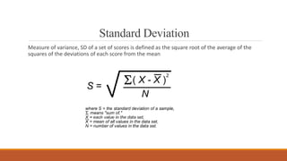
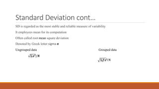
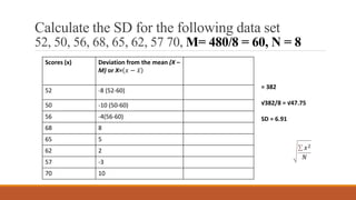
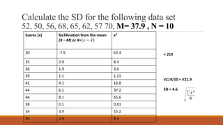
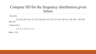
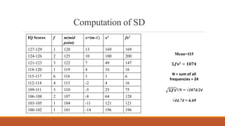
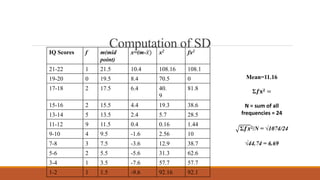
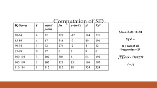
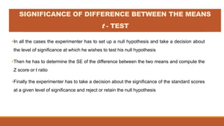
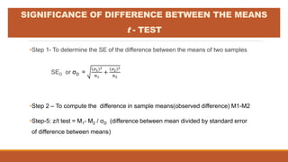
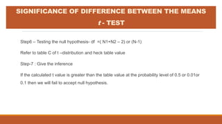
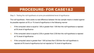
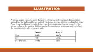
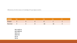
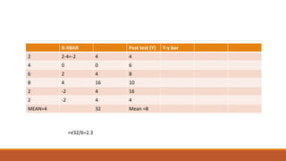
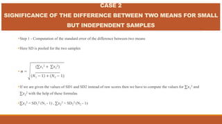
Standard deviation (SD) is a measure of variability or dispersion of data from the mean. It is calculated as the square root of the average of the squared deviations from the mean. The t-test is used to determine if there is a statistically significant difference between the means of two groups, and requires calculation of the standard error of the difference between the means. There are different procedures for the t-test depending on whether the samples are independent or correlated, large or small. The null hypothesis of no difference between means is tested against the alternative hypothesis at a chosen significance level.

1. STANDARD DEVIATION
AND
‘t’- TEST
Keerthi Samuel

2. DIFFERENCE BETWEEN PARAMETRIC AND
NON PARAMETRIC STATISTICS
PARAMETRIC NON-PARAMETRIC
The data should be normally distributed Distribution free(skewed, outliers)
Homogeneity of variance Homogeneous or heterogeneous
Ratio or interval data Nominal or ordinal data
Independent data Any
Measure of central tendency - Mean Measure of central tendency – Median
Sample size should be large Small sample size
Useful in drawing conclusions and generalizations Simple and less effective
t-test, ANOVA, Pearson’s correlation, MANOVA, ANCOVA,
Regression
Chi-square, Mann Whitney U test, Sign test, Kruskal wallis
test, Spearman's Rho

3. Standard Deviation
Measure of variance, SD of a set of scores is defined as the square root of the average of the
squares of the deviations of each score from the mean

4. Standard Deviation cont…
SD is regarded as the most stable and reliable measure of variability
It employees mean for its computation
Often called root mean square deviation
Denoted by Greek letter sigma σ
Ungrouped data Grouped data
Σ𝒙𝟐/𝑵
Σ𝒇𝒙2/N

5. Standard Deviation cont…
SD is regarded as the most stable and reliable measure of variability
It employees mean for its computation
Often called root mean square deviation
Denoted by Greek letter sigma σ
Ungrouped data Grouped data
Σ𝑿𝟐/𝑵
Σ𝒇𝒙2/N

6. Calculate the SD for the following data set
52, 50, 56, 68, 65, 62, 57 70, M= 480/8 = 60, N = 8
Scores (x) Deviation from the mean (X –
M) or X= 𝑥 − 𝑥
x2
52 -8 (52-60) 64
50 -10 (50-60) 100
56 -4(56-60) 16
68 8 64
65 5 25
62 2 4
57 -3 9
70 10 100
= 382
√382/8 = √47.75
SD = 6.91
𝑥2
𝑁

7. Calculate the SD for the following data set
52, 50, 56, 68, 65, 62, 57 70, M= 37.9 , N = 10
Scores (x) De34viation from the mean
(X – M) or X= 𝑥 − 𝑥
x2
30 -7.9 62.4
35 2.9 8.4
36 1.9 3.6
39 1.1 1.21
42 4.1 16.8
44 6.1 37.2
46 8.1 65.6
38 0.1 0.01
34 3.9 15.2
35 2.9 8.4
= 219
√219/10 = √21.9
SD = 4.6
𝑥2
𝑁

8. Compute SD for the frequency distribution given
below
IQ scores :
127-129, 124-126, 121-123, 118-120, 115-117, 112-114, 109-111, 106-108, 103-105,
100-102
Frequencies :
1, 2, 3, 1, 6, 4, 3, 2, 1, 1
Mean - 115

9. Computation of SD
IQ Scores f m(mid
point)
x=(m-𝑥) x2 fx2
127-129 1 128 13 169 169
124-126 2 125 10 100 200
121-123 3 122 7 49 147
118-120 1 119 4 16 16
115-117 6 116 1 1 6
112-114 4 113 -2 4 16
109-111 3 110 -5 25 75
106-108 2 107 -8 64 128
103-105 1 104 -11 121 121
100-102 1 101 -14 196 196
Mean=115
Σ𝒇𝐱𝟐 = 𝟏𝟎𝟕𝟒
N = sum of all
frequencies = 24
Σ𝒇𝒙2/N = √1074/24
√44.74 = 6.69

10. Computation of SD
IQ Scores f m(mid
point)
x=(m-𝑥) x2 fx2
21-22 1 21.5 10.4 108.16 108.1
19-20 0 19.5 8.4 70.5 0
17-18 2 17.5 6.4 40.
9
81.8
15-16 2 15.5 4.4 19.3 38.6
13-14 5 13.5 2.4 5.7 28.5
11-12 9 11.5 0.4 0.16 1.44
9-10 4 9.5 -1.6 2.56 10
7-8 3 7.5 -3.6 12.9 38.7
5-6 2 5.5 -5.6 31.3 62.6
3-4 1 3.5 -7.6 57.7 57.7
1-2 1 1.5 -9.6 92.16 92.1
Mean=11.16
Σ𝒇𝐱𝟐 =
N = sum of all
frequencies = 24
Σ𝒇𝒙2/N = √1074/24
√44.74 = 6.69

11. Computation of SD
IQ Scores f m(mid
point)
fm x=(m-𝑥) x2 Fx2/
80-84 4 82 328 -12 144 576
85-89 4 87 348 -7 49 196
90-94 3 92 276 -2 4 12
95-99 0 97 0 3 9 0
100-104 3 102 306 8 64 192
105-109 3 107 321 13 169 507
110-114 1 112 112 18 324 324
Mean=1691/18=94
Σ𝒇𝐱𝟐 =
N = sum of all
frequencies = 24
Σ𝒇𝒙2/N = √1807/18
√ = 10

12. When to use Standard Deviation
When we need a most reliable measure of variability
If there is a need of computation of the correlation coefficients, significance of difference
between means
Measure of central tendency is available in the form of mean
The distribution is normal

13. Compute SD for the following
1. 30, 35, 36, 39, 42, 44, 46, 38, 34, 35
2. 80-84, 85-89, 90-94, 95-99, 100-104, 105-109, 110-114 ; F – 4, 4, 3, 0, 3, 3, 1
3. Scores : 21-22, 19-20, 17-18, 15-16, 13-14, 11-12, 9-10, 7-8, 5-6, 3-4, 1-2
F – 1, 0, 2, 2, 5, 9, 4, 3, 2, 1, 1

14. SIGNIFICANCE OF DIFFERENCE BETWEEN THE MEANS
‘t ‘- TEST
The process of determining the difference between two given sample means varies with respect
to the size of the group
Case 1 – large but independent samples
Case 2 – small but independent samples
Case 3 – large but correlated samples
Case 4 – small but correlated samples

15. Paired- X1PRETEST LSCS-------O(ONINE CLASS)----------X2 POST TEST
DEGREE OF FREEDOM=n-1
UNPAIRED –XI LSCS-----------O-------------X2 (30)
Y1 FTND-----------------O1------------------Y2(30)
EFDECCTIVENESS OF WALKING ON INVOLUTION OF UTERUS AMONG LSCS MOTHERS
Df=n1+n2-2
30+30-2

16. •In all the cases the experimenter has to set up a null hypothesis and take a decision about
the level of significance at which he wishes to test his null hypothesis
•Then he has to determine the SE of the difference between the two means and compute the
Z score or t ratio
•Finally the experimenter has to take a decision about the significance of the standard scores
at a given level of significance and reject or retain the null hypothesis
SIGNIFICANCE OF DIFFERENCE BETWEEN THE MEANS
t - TEST

17. •Step 1- To determine the SE of the difference between the means of two samples
SED or σD =
𝜎1
2
𝑛1
+
𝜎2
2
𝑛2
•Step 2 – To compute the difference in sample means(observed difference) M1-M2
•Step-5: z/t test = M1- M2 / σD (difference between mean divided by standard error
of difference between means)
SIGNIFICANCE OF DIFFERENCE BETWEEN THE MEANS
t - TEST

18. Step6 – Testing the null hypothesis- df =( N1+N2 – 2) or (N-1)
Refer to table C of t –distribution and heck table value
Step-7 : Give the inference
If the calculated t value is greater than the table value at the probability level of 0.5 or 0.01or
0.1 then we will fail to accept null hypothesis.
SIGNIFICANCE OF DIFFERENCE BETWEEN THE MEANS
t - TEST

19. PROCEDURE- FOR CASE1&2
Step 3 - Testing the null hypothesis at some pre-established level of significance
The null hypothesis - there exists no real difference between the two sample means is tested against
its possible rejection at 5% or 1% level of significance in the following manner
i) If the computed value is equal to 1.96 or greater than 1.96 then the null hypothesis is rejected
at 5% level of significance
ii) If the computed value is equal to 2.58 or greater than 2.58 then the null hypothesis is rejected
at 1% level of significance
iii) If the computed value is greater than 1.96 but less than 2.58 then the null hypothesis is
rejected at 5% level of significance but not rejected at 1% level of significance

20. ILLUSTRATION
A science teacher wanted to know the relative effectiveness of lecture cum demonstration
method over the traditional lecture method. He divided his class into two equal random group
A and B and taught group A by the lecture cum demonstration method and group B by the
lecture method. After teaching for three months he administered an achievement test to both
the groups the data collected were as under
Group A Group B
Mean 43(M1) 30(M2)
SD 8(SD1) 7(SD2)
No. of students 65(n1) 65(n2)

21. Effectiveness of online classes on knowledge of III year degree students
MARKS A B C D E F
Pretest 2 4 6 8 2 2
Post test 4 6 8 10 16 4
M1=24/6=4
M2=48/6=8
SD1=2.3
SD2=4.6
N1=6
N2=6

22. X-XBAR Post test (Y) Y-y bar
2 2-4=-2 4 4
4 0 0 6
6 2 4 8
8 4 16 10
2 -2 4 16
2 -2 4 4
MEAN=4 32 Mean =8
=√32/6=2.3

23. CASE 2
SIGNIFICANCE OF THE DIFFERENCE BETWEEN TWO MEANS FOR SMALL
BUT INDEPENDENT SAMPLES
•Step 1 - Computation of the standard error of the difference between two means
•Here SD is pooled for the two samples
• σ =
( 𝑥1
2 + 𝑥2
2)
_________________
𝑁1 − 1 + (𝑁2 − 1)
•If we are given the values of SD1 and SD2 instead of raw scores then we have to compute the values for 𝑥1
2 and
𝑥2
2 with the help of these formulas
• 𝑥1
2 = SD1
2 (N1 - 1) , 𝑥2
2 = SD2
2 (N2 - 1)

24. ILLUSTRATION
Group 1 – 10, 9, 8, 7, 7, 8, 6, 5, 6, 4
Group 2 – 9,8, 6, 7, 8, 8, 11, 12, 6, 5
Find M1 and M2, find pooled SD, t and df

25. ILLUSTRATION
X1 M1 x1 x1
2 X2 M2 x2 x2
2
10 7 3 9 9 8 1 1
9 7 2 4 8 8 0 0
8 7 1 1 6 8 -2 4
7 7 0 0 7 8 -1 1
7 7 0 0 8 8 0 0
8 7 1 1 8 8 0 0
6 7 -1 1 11 8 3 9
5 7 -2 4 12 8 4 16
6 7 -1 1 6 8 -2 4
4 7 -3 9 5 8 -3 9

26. PRACTICE
A language teacher divides the class into two groups experimental group and control group.
Under the assumption that newspaper reading will increase the vocabulary the experimental
group was given two hours daily to read English newspapers and magazines while no such
facility was provided to the control group. After 6 months both the groups were given a
vocabulary test and the scores obtained are detailed below
Experimental group – 115, 112, 109, 112, 137
Control group – 110, 112, 95, 105, 111, 97, 112,102

27. CASE 3 AND 4
SIGNIFICANCE OF THE DIFFERENCE BETWEEN TWO MEANS FOR
CORRELATED SAMPLES – LARGE AND SMALL
•Single group method – Repetition of a test to a group of subjects called the initial test
then the desired experiment (intervention) is given, followed by the same test to the
same individuals
•The initial and final test data are correlated
•σD = √σM1
2+σM2
2 − 2rσM1σM2
•σM1 = Standard error of the initial test, σM2 = Standard error of the final test
•r = coefficient of correlation between scores on initial and final testing

28. •Equivalent group method – When we have to compare relative effect of one method or
treatment over the other with two groups (experimental and control)
•Matching pair technique – Matching is done before the initial test in which each
individual is paired with an equivalent match in the other group in terms of variables
that are going to affect the results of the study such as age, socio economic
background, intelligence etc.
•Matching group technique – the group as a whole is matched with another group in
terms of their mean, SD.
CASE 3 AND 4
SIGNIFICANCE OF THE DIFFERENCE BETWEEN TWO MEANS
FOR CORRELATED SAMPLES – LARGE AND SMALL

29. In case of grouped matched data the formula is
σD = √(σM1
2+σM2
2 ) (1−r2)
Illustration :
Initial test mean = 70, SD = 6
Final test mean = 67,SD = 5.8
r = 0.82
CASE 3 AND 4
SIGNIFICANCE OF THE DIFFERENCE BETWEEN TWO MEANS FOR
CORRELATED SAMPLES – LARGE AND SMALL