This document discusses frequency distributions, which organize and simplify data by tabulating how often values occur within categories. Frequency distributions can be regular, listing all categories, or grouped, combining categories into intervals. They are presented in tables showing categories/intervals and frequencies. Graphs like histograms and polygons also display distributions. Distributions describe data through measures of central tendency, variability, and shape. Percentiles indicate the percentage of values at or below a given score.

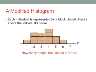
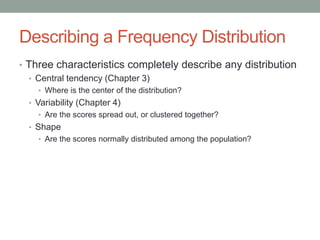
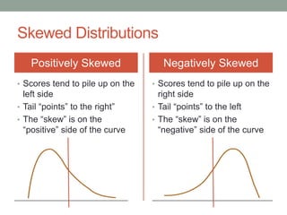
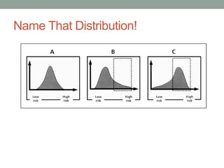
1. FREQUENCY
DISTRIBUTIONS
Behavioral Statistics
Summer 2017
Dr. Germano

2. What is a frequency distribution?
An organized tabulation of the number of individuals
located in each category on a scale of measurement
• A method for simplifying and organizing
data
• Presents an organized picture of the
entire set of scores
• Are scores generally high or low?
• Are the scores clustered together or spread
out?
• Shows where each individual is located
relative to others in a distribution
• Where does one score fall relative to all
others?

3. Frequency Distribution Tables
• Consists of at least two columns
• Categories on the scale of measurement (X), ordered from lowest to
highest
• Frequency for each category (how often each category was reported)
Original scores: 1, 2, 3, 5, 4, 4, 2, 3, 1, 3, 2, 3, 2, 2
Frequency table:
1 was the lowest reported
score. Two people had a
score of 1.
2 was the most commonly
reported score. Five
people had a score of 2.

4. Frequency Distributions: Obtaining N
• N = the number of observations
(or, number of cases)
• Remember your notations:
• Score = X
• Frequency = f
• Thus, N = Σf
X f
1 2
2 5
3 4
4 2
5 1
Σf = 14
Σf = 2 + 5 + 4 + 2 + 1
Σf = 14

5. Frequency Distributions: Obtaining ΣX
• Remember your notations:
• Score = X
• Frequency = f
• How do we get ΣX?
• Add up all the scores
• Multiply each score by the
frequency and add up the results
X f
1 2
2 5
3 4
4 2
5 1
Σf = 14
Xf
2 x 1 = 2
2 x 5 = 10
3 x 4 = 12
4 x 2 = 8
5 x 1 = 5
ΣX = 37
ΣX = 1 + 1 + 2 + 2 + 2 + 2 + 2 + 3 + 3 + 3 + 3 + 4 + 4 + 5
ΣX = 37

6. Obtaining (ΣX)2 and ΣX2
X f
1 2
2 5
3 4
4 2
5 1
Σf = 14
ΣX2 = 12+ 12+ 22+ 22+ 22+ 22+ 22+ 32+ 32+ 32+ 32+ 42+ 42+ 52
ΣX2 = 1 + 1 + 4 + 4 + 4 + 4 + 4 + 9 + 9 + 9 + 9 + 16 + 16 + 25
ΣX2 = 115
• Remember the order of operations:
1. Parentheses
2. Exponents
3. Multiplication/Division
4. Adding/Subtracting
(ΣX)2 = (37)2
(ΣX)2 =1369

7. Proportions (p) and Percentages (%)
• p measures the fraction of the total group
associated with each score
• p = f/N
X f
1 2
2 5
3 4
4 2
5 1
Σf = 14
p = f/N
2/14 = 0.143
5/14 = 0.357
4/14 = 0.286
2/14 = 0.143
1/14 = 0.071
% = p(100)
14.3%
35.7%
28.6%
14.3%
7.1%
Σp = 1.00 Σ% = 100%
*Math check: sum proportions = 1.00;
sum percentages = 100%

8. Types of Frequency Distribution Tables
Regular Frequency Distribution
• Lists all of the individual
categories (X values)
Grouped Frequency Distribution
• When listing all of the
individual categories is
not
possible/helpful/reasonabl
e
• e.g., Test scores 0-100
X f
1 2
2 5
3 4
4 2
5 1
Σf = 14

9. Grouped Frequency Tables
• Range of scores on a test: 39 – 85
• Organized by class intervals
• More efficient
• Guidelines
1. No more than 10 class intervals
2. Width of each interval should be a
simple number (i.e., 2, 5, 10, 20)
3. Bottom score of each interval should be a multiple of
the width (in this case, a multiple of “10”)
4. All intervals should be equal
X f
80-89 4
70-79 6
60-69 12
50-59 8
40-49 4
30-39 2

10. Grouped Frequency Tables
• What information is lost?
• The individual scores – and thus, our
ability to solve for Σ(Xf)
X f
80-89 4
70-79 6
60-69 12
50-59 8
40-49 4
30-39 2

11. Constructing a Grouped Frequency Table
For a set of N = 25 scores: 82, 75, 88, 93, 53,
84, 87, 58, 72, 94,
69, 84, 61, 91, 64,
87, 84, 70, 76, 89,
75, 80, 73, 78, 60

12. Constructing a Grouped Frequency Table
For a set of N = 25 scores: 82, 75, 88, 93, 53,
84, 87, 58, 72, 94,
69, 84, 61, 91, 64,
87, 84, 70, 76, 89,
75, 80, 73, 78, 60
1. Determine the range of scores
• Range = 42
Smallest score is X = 53
Largest score is X = 94
94 - 53 = 42

13. Constructing a Grouped Frequency Table
For a set of N = 25 scores: 82, 75, 88, 93, 53,
84, 87, 58, 72, 94,
69, 84, 61, 91, 64,
87, 84, 70, 76, 89,
75, 80, 73, 78, 60
1. Determine the range of scores
• Range = 42
2. Group scores into intervals
• At least 9 intervals needed
Smallest score is X = 53
Largest score is X = 94
94 - 53 = 42
Width # of Intervals Needed to
Cover a Range of 42 Points
2 21 (too many)
5 9 (OK)
10 5 (too few)

14. Constructing a Grouped Frequency Table
For a set of N = 25 scores: 82, 75, 88, 93, 53,
84, 87, 58, 72, 94,
69, 84, 61, 91, 64,
87, 84, 70, 76, 89,
75, 80, 73, 78, 60
1. Determine the range of scores
• Range = 42
2. Group scores into intervals
• At least 9 intervals needed
3. Identify the intervals
• Bottom interval should be
50-54
• Next is 55-59
• Then 60-64
• Etc.
Smallest score is X = 53
Largest score is X = 94
94 - 53 = 42
Lowest score is X = 53
Lowest interval should contain this value
Interval should have a multiple of 5 as its
bottom score
Interval should contain 5 values (because
it has an interval of 5)

15. Constructing a Grouped Frequency Table
For a set of N = 25 scores:
1. Determine the range of scores
• Range = 42
2. Group scores into intervals
• At least 9 intervals needed
3. Identify the intervals
• Bottom interval should be
50-54
• Next is 55-59
• Then 60-64
• Etc.
X
90-94
85-89
80-84
75-79
70-74
65-69
60-64
55-59
50-54
f
3
4
5
4
3
1
3
1
1
p = f/N
0.12
0.16
0.20
0.16
0.12
0.04
0.12
0.04
0.04
Σp
1.00
Σ%
100%
%
12%
16%
20%
16%
12%
4%
12%
4%
4%

16. Real Limits
Recall from Chapter 1:

17. Real Limits and Frequency Distributions
X
90-94
85-89
80-84
75-79
70-74
65-69
60-64
55-59
50-54
f
3
4
5
4
3
1
3
1
1
• For X = 60 – 64, there are 3 scores
• Does not mean 3 scores are identical
• Means 3 scores fall within the interval
• For each interval, there are limits
• Lower real limit
• Upper real limit 3 different scores
within this interval
50 55 60 65 70 75 80 85 90 95
59.5 – 64.5
Apparent Limits
Real Limits

18. Frequency Distribution Graphs
• X-axis (abscissa)
• Horizontal line
• Values increase from left to right
• Y-axis (ordinate)
• Vertical line
• Values increase from bottom to
top
• In a frequency distribution graph:
• Score categories (X values) are listed on the X axis
• Frequencies are listed on the Y axis

19. Graphs for Interval or Ratio Data
Histogram
• Adjacent bars touch
• Height of bar indicates
frequency
• Width corresponds to the score
(or limits of the range of scores)
Polygon
• Vertical position of dot indicates a
score’s frequency
• Continuous line is draw between
series of dots
• X = 0 typically one category
above/below highest/lowest score

20. A Modified Histogram
• Each individual is represented by a block placed directly
above the individual’s score.
How many people had scores of X = 2?

21. Histogram and Polygon on One Graph

22. What If Your Data Is Not Interval/Ratio?
• Bar Graph
• For nominal or ordinal data
• Like a histogram in structure, but the bars do not touch
• Emphasizes distinct categories

23. Leave NYC
immediately!
A Warning…

24. Don’t Misrepresent Your Data!
Leave NYC
immediately!
Oh, wait…
A Warning…

25. Graphs for Population Distributions
Relative Frequencies
• We may not know exactly how
many fish are in Lake Erie, but
we do know that there are
double the number of Bluegill
than there are Bass
Smooth Curves
• When the population consists of
numerical scores from an interval
or ratio scale
• Indicates that we are showing the
relative changes that occur from
one score to the next

26. Describing a Frequency Distribution
• Three characteristics completely describe any distribution
• Central tendency (Chapter 3)
• Where is the center of the distribution?
• Variability (Chapter 4)
• Are the scores spread out, or clustered together?
• Shape
• Are the scores normally distributed among the population?

27. The Shape of a Frequency Distribution

28. Skewed Distributions
Positively Skewed
• Scores tend to pile up on the
left side
• Tail “points” to the right”
• The “skew” is on the
“positive” side of the curve
Negatively Skewed
• Scores tend to pile up on the
right side
• Tail “points” to the left
• The “skew” is on the
“negative” side of the curve

29. Name That Distribution!

30. Name That Distribution!
Symmetric (no skew) Positive Skew Negative Skew

31. Percentiles & Percentile Ranks
• Percentile rank
• The percentage of individuals in the distribution with scores at or
below the particular value
• Percentile
• When a score is identified by its percentile rank
For example:
o Your exam score is X = 43
o 60% of the class had scores of 43 or lower
o Your score has a percentile rank of 60% and is called the 60th
percentile.

32. Percentiles & Percentile Ranks
X f Xf p % cf c%
1 2 2 0.143 14.3% 2 (2/14)100% = 14.3%
2 5 10 0.357 35.7% (2+5) = 7 (7/14)100% = 50%
3 4 12 0.286 28.6% (7+4) = 11 (11/14)100% = 78.6%
4 2 8 0.143 14.3% (11+2) = 13 (13/14)100% = 92.9%
5 1 5 0.071 7.1% (13+1) = 14 (14/14)100% = 100%
N = 14 (x lowx high) (cf/N)(100%)
• To find percentiles and percentile ranks, we must first
calculate cumulative frequency (cf) and cumulative
percentage (c%) for each score (or interval)

33. Let’s Practice
1. Find the 70th percentile (remember real limits!)
2. Find the percentile rank for X = 9.4
X f cf c%
0 – 4 2 2 10%
5 – 9 4 6 20%
10 – 14 8 14 70%
15 – 19 5 19 95%
20 - 24 1 20 100%