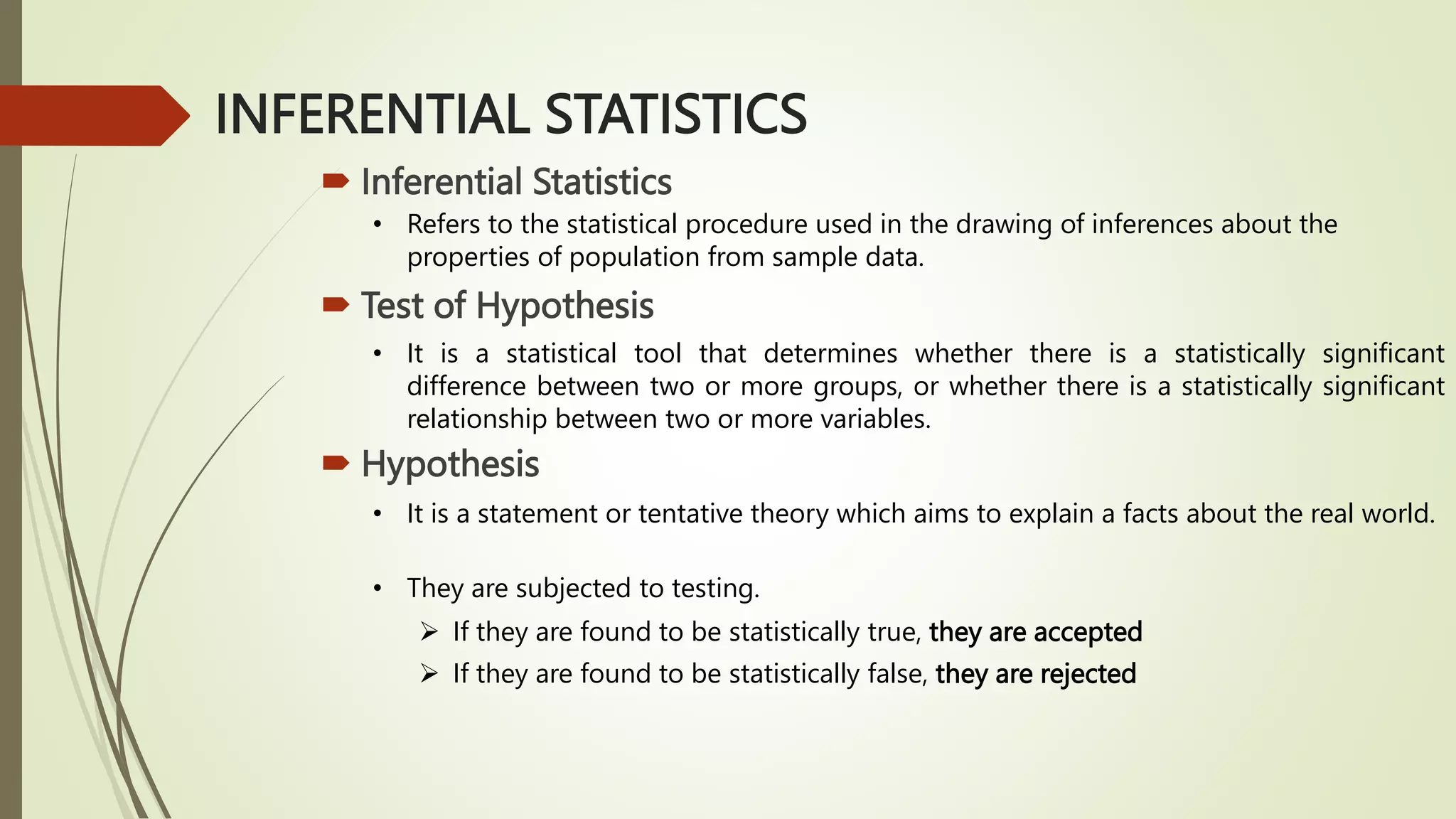
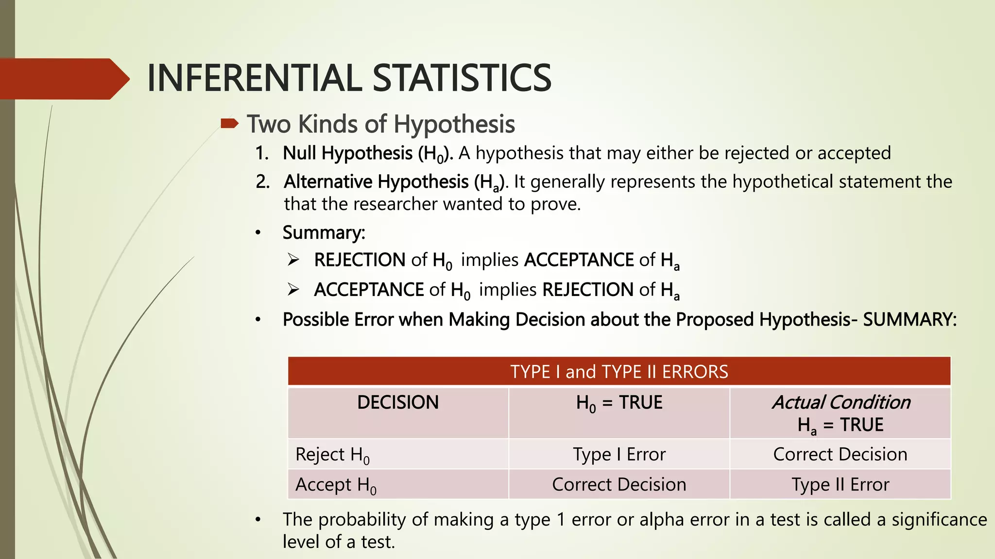
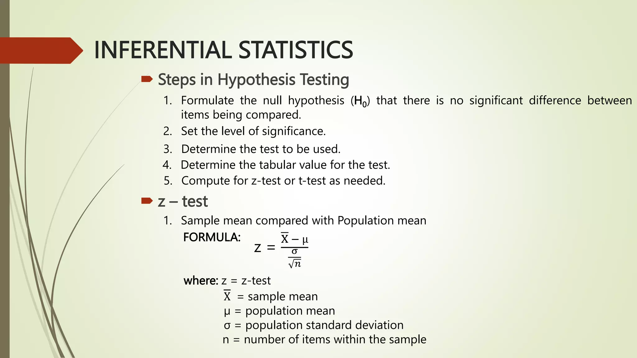
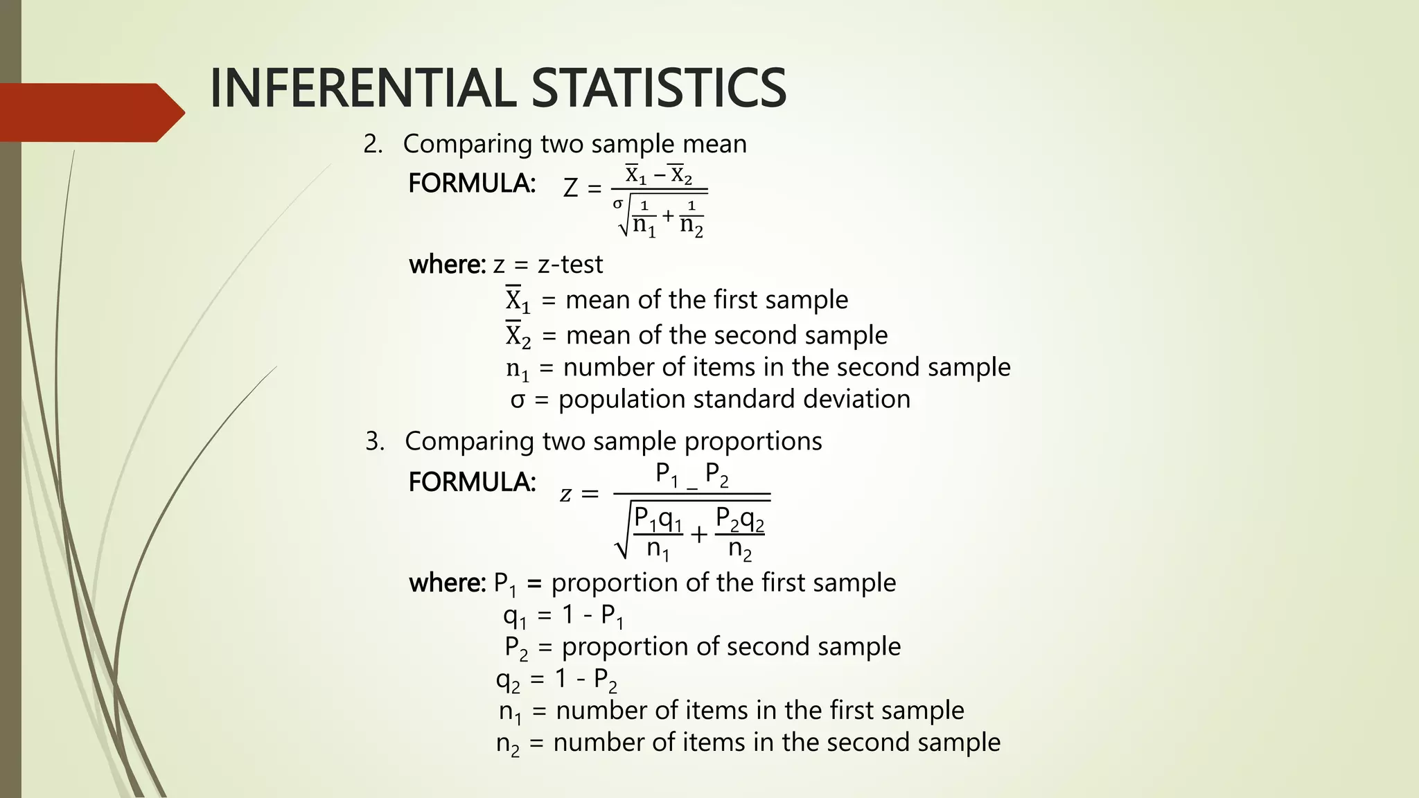
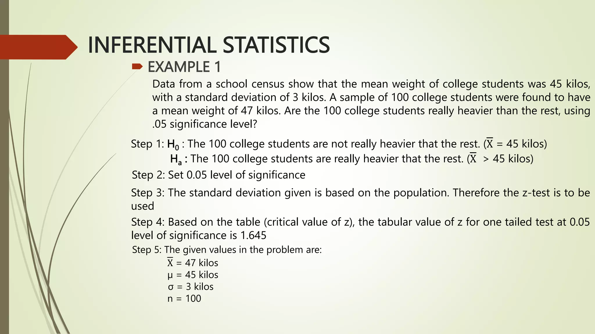
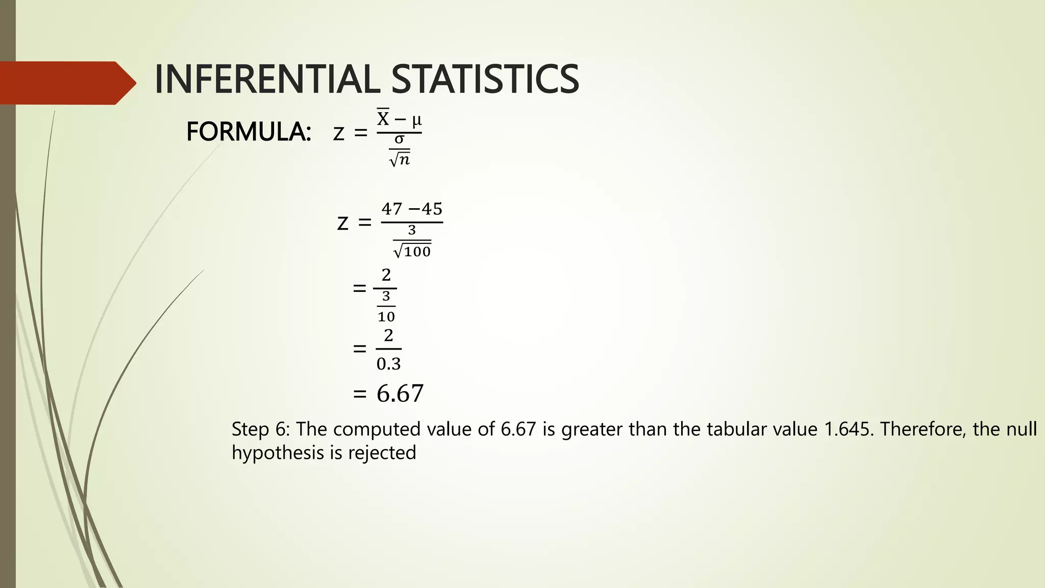
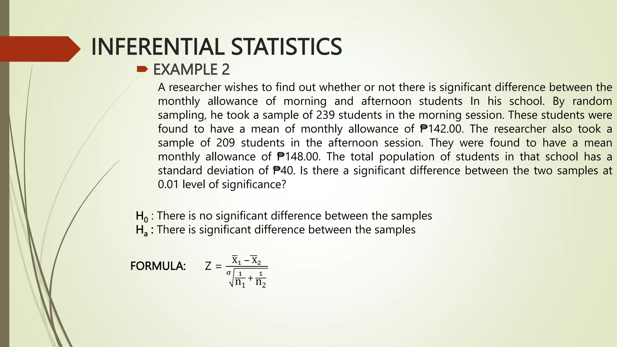
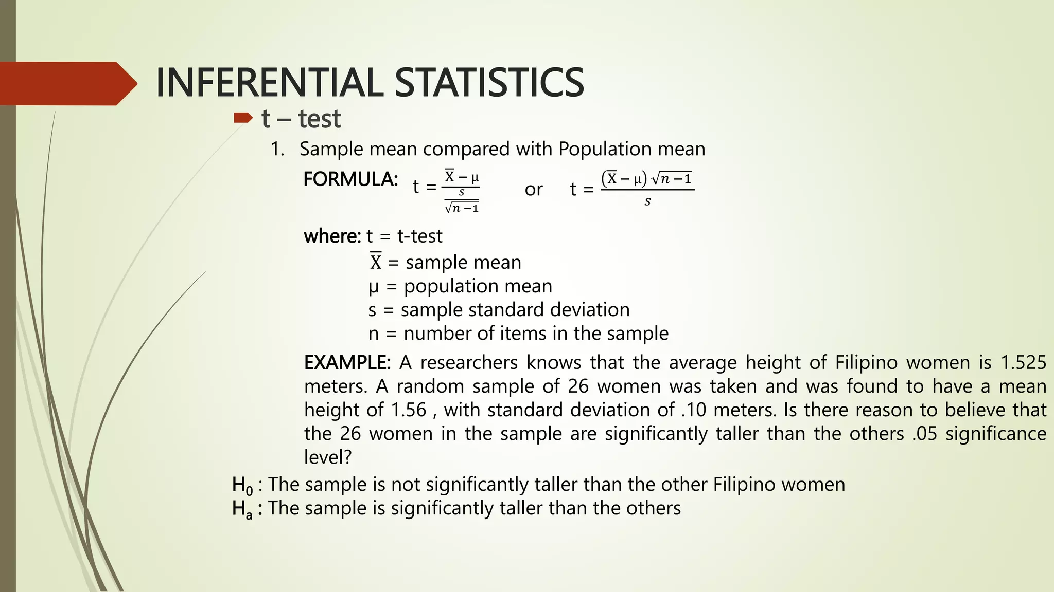
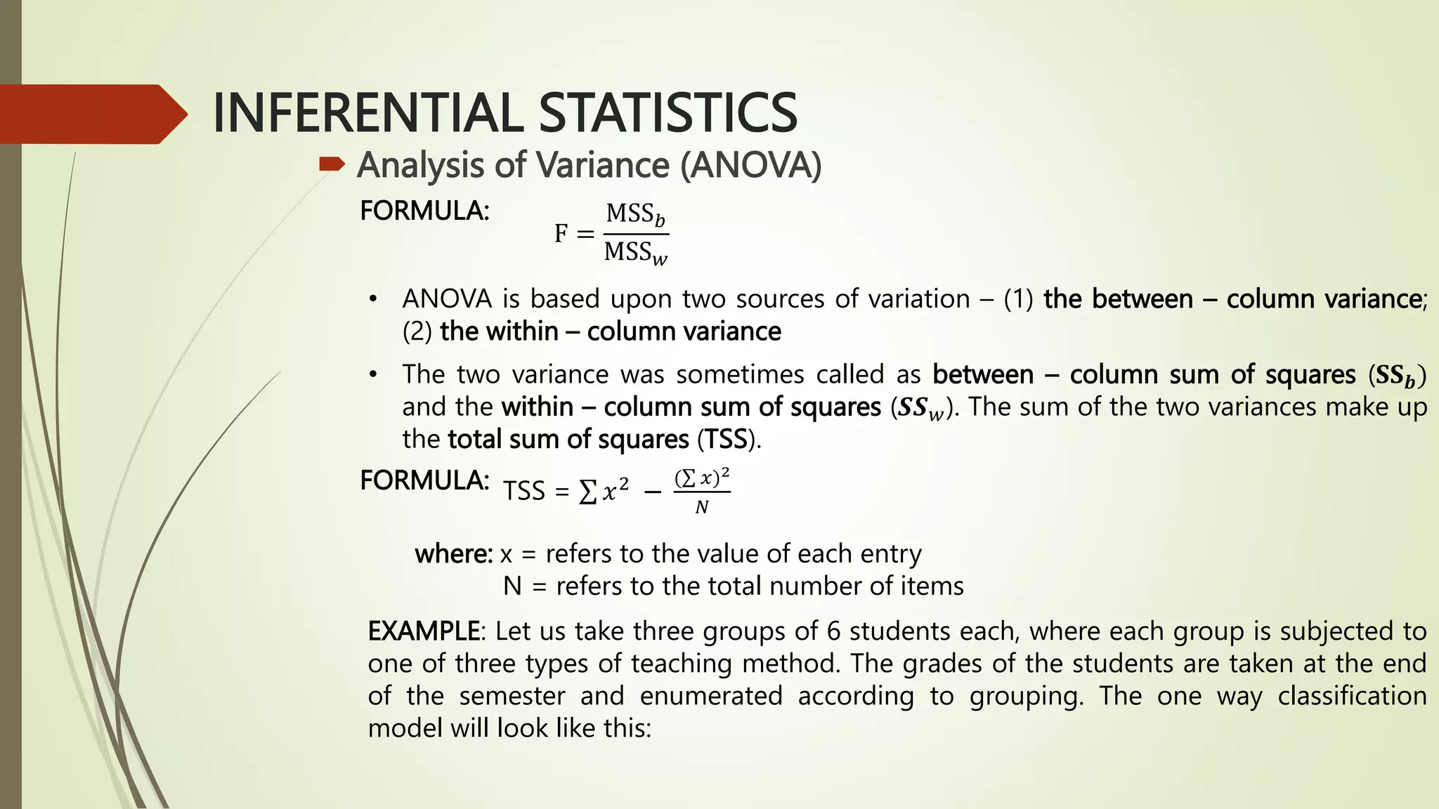
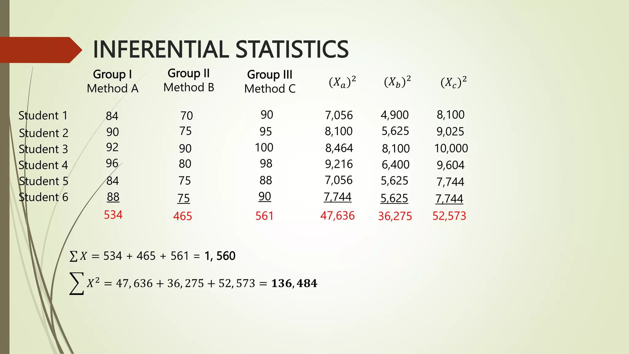
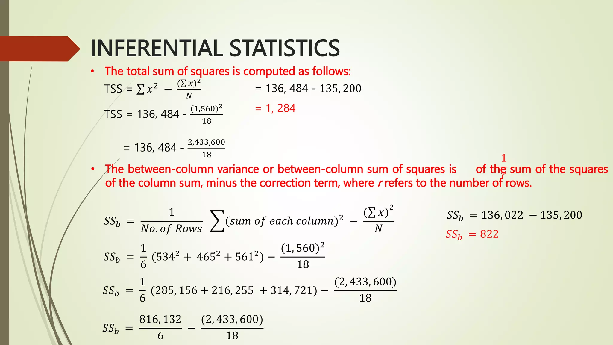
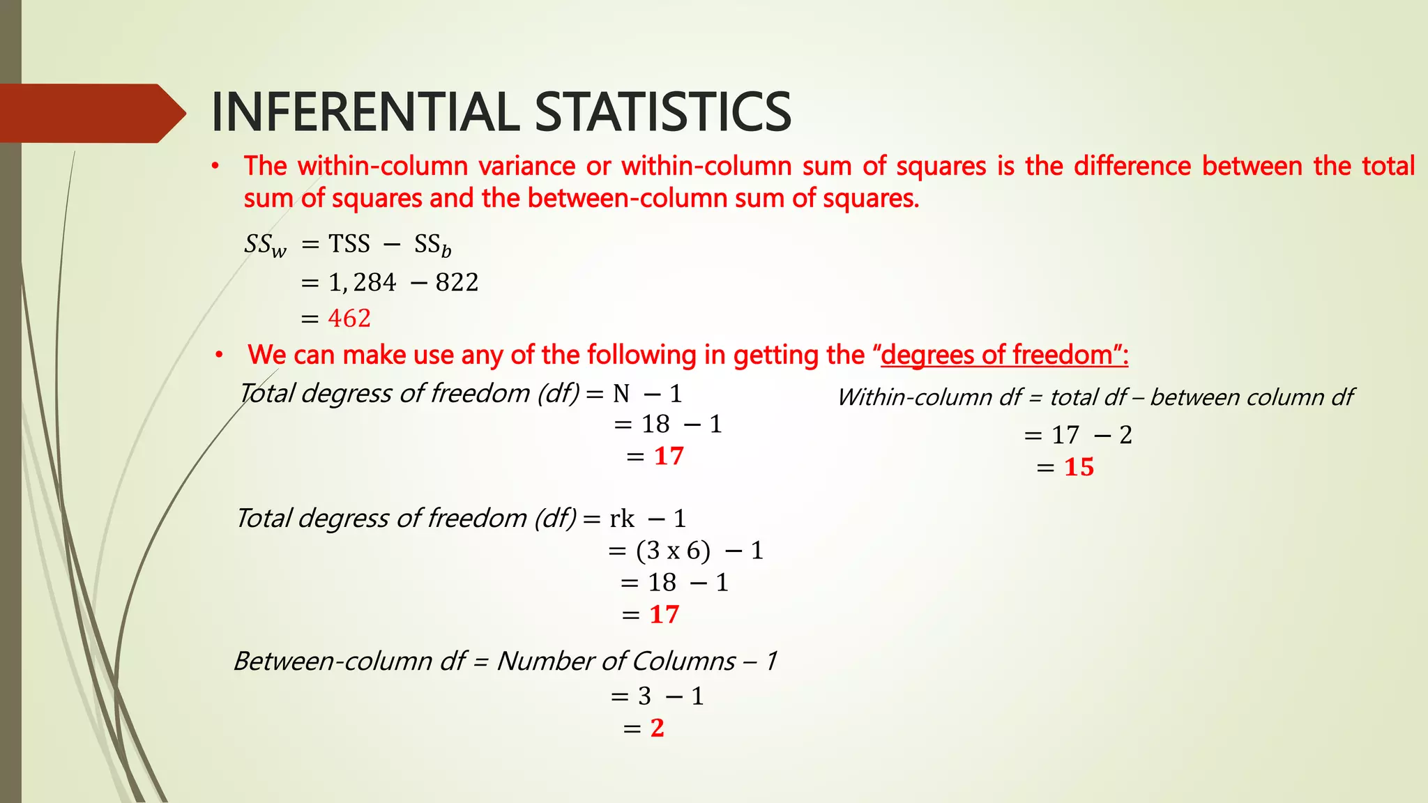
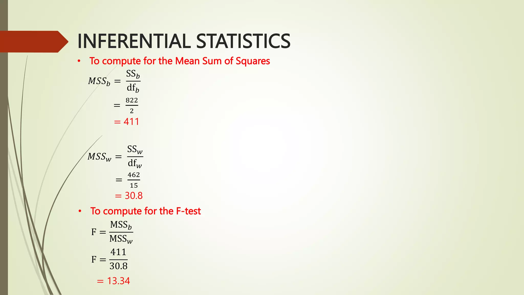
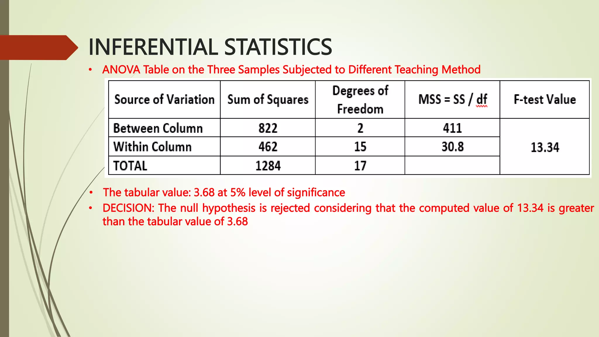
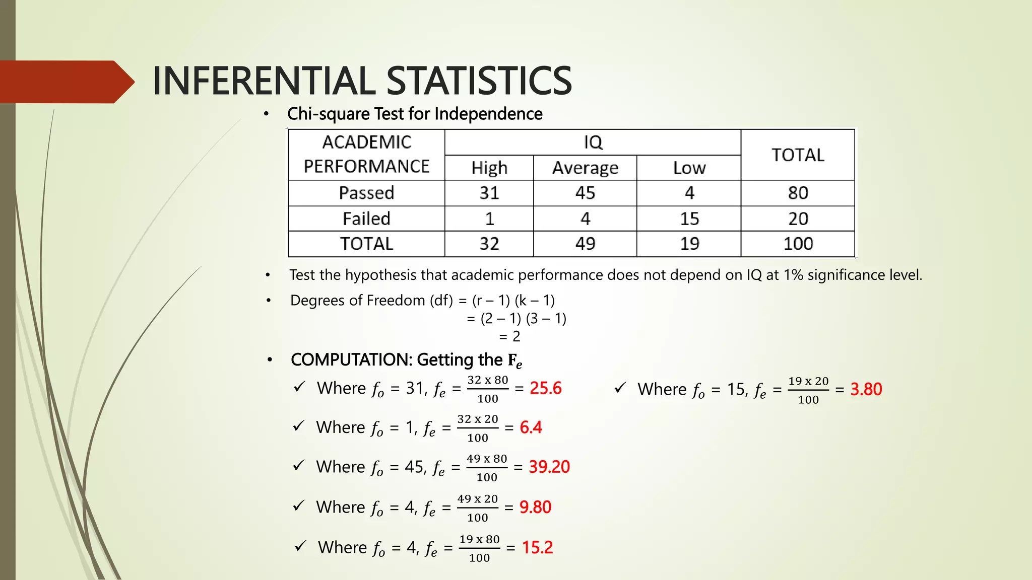
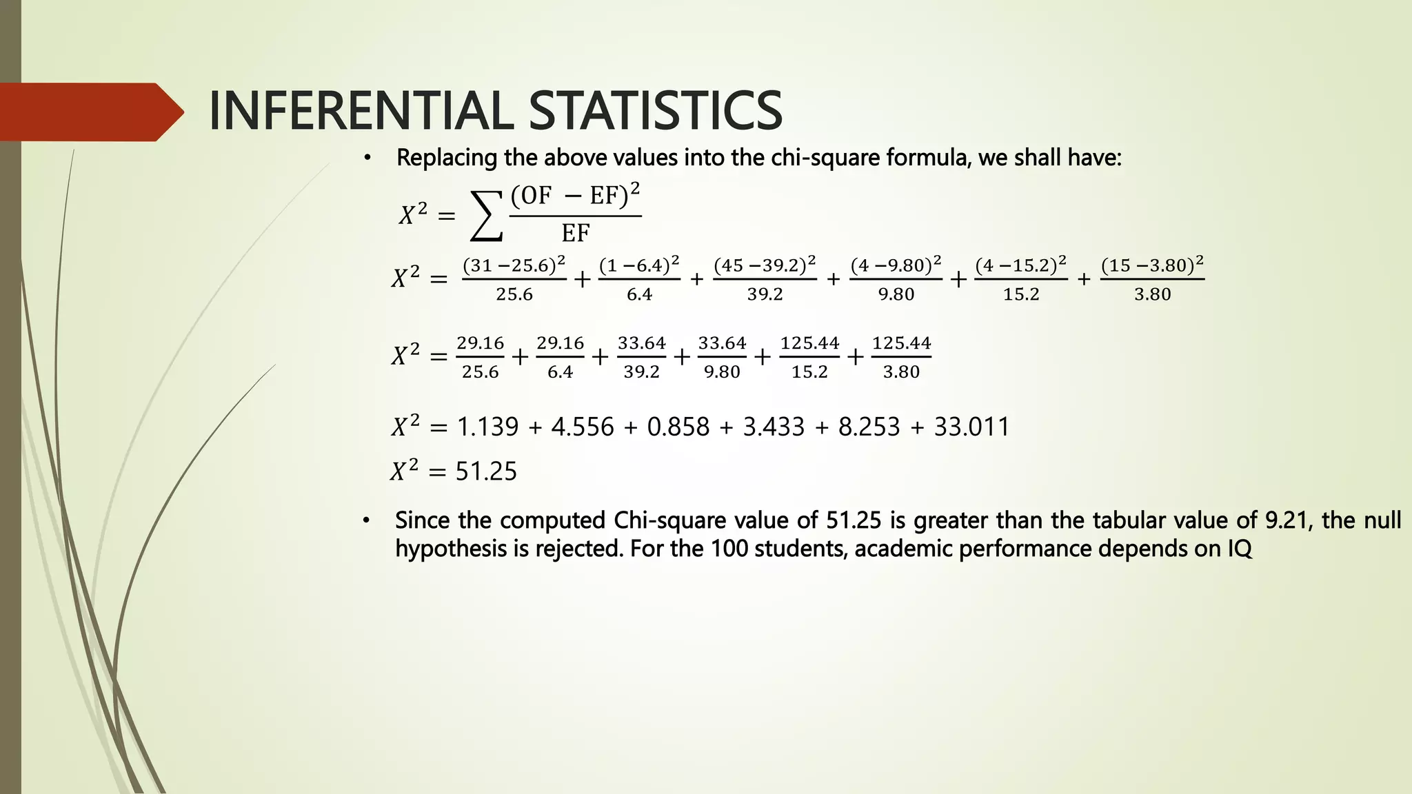
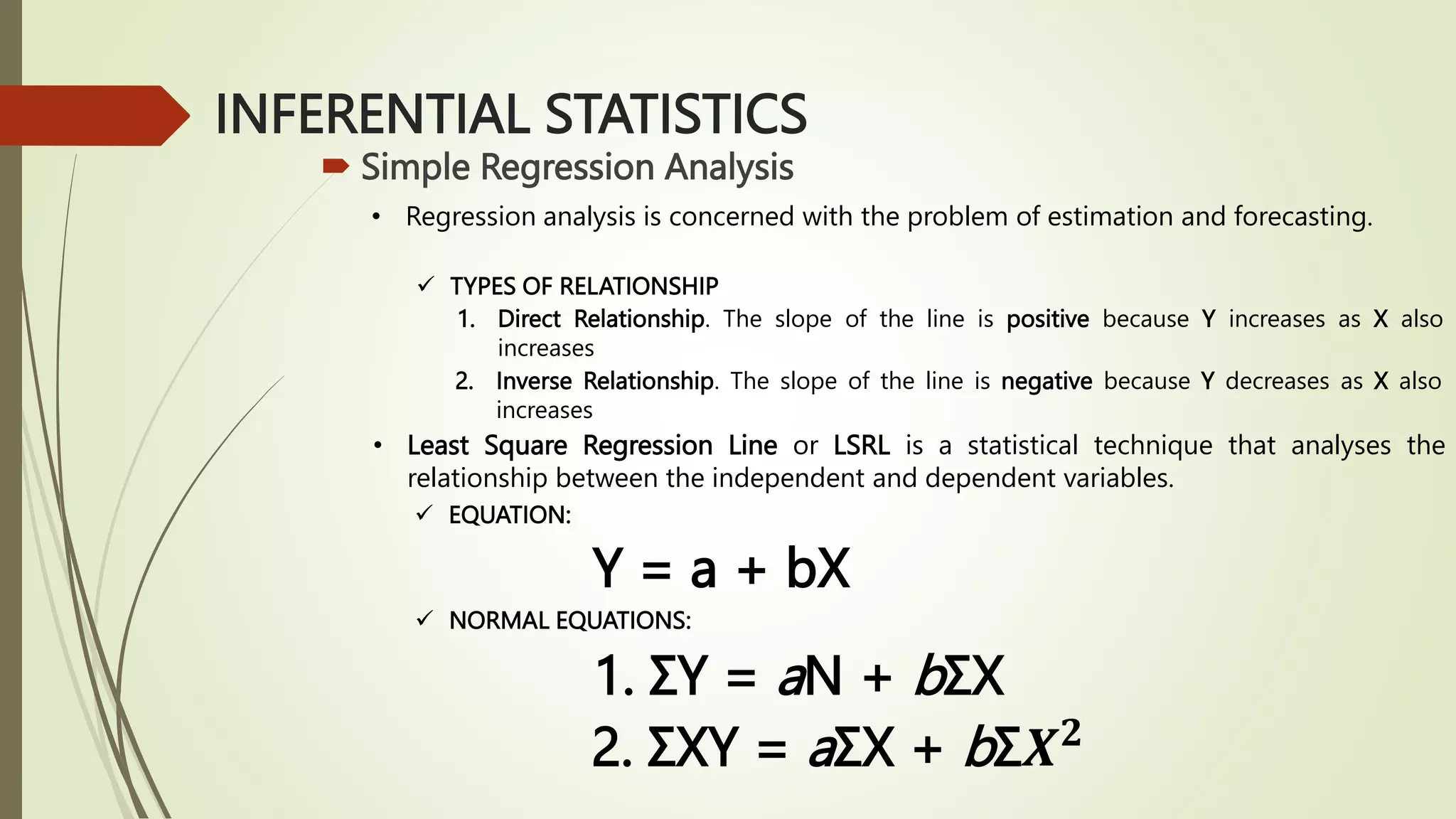
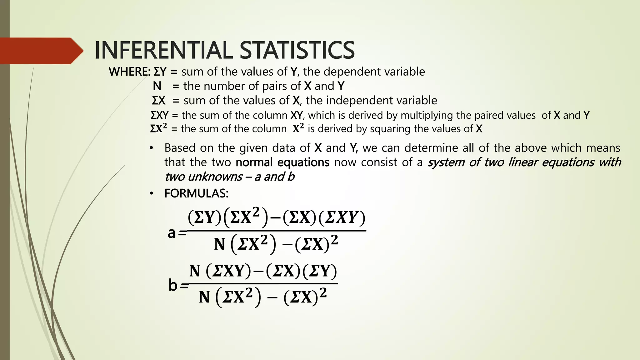
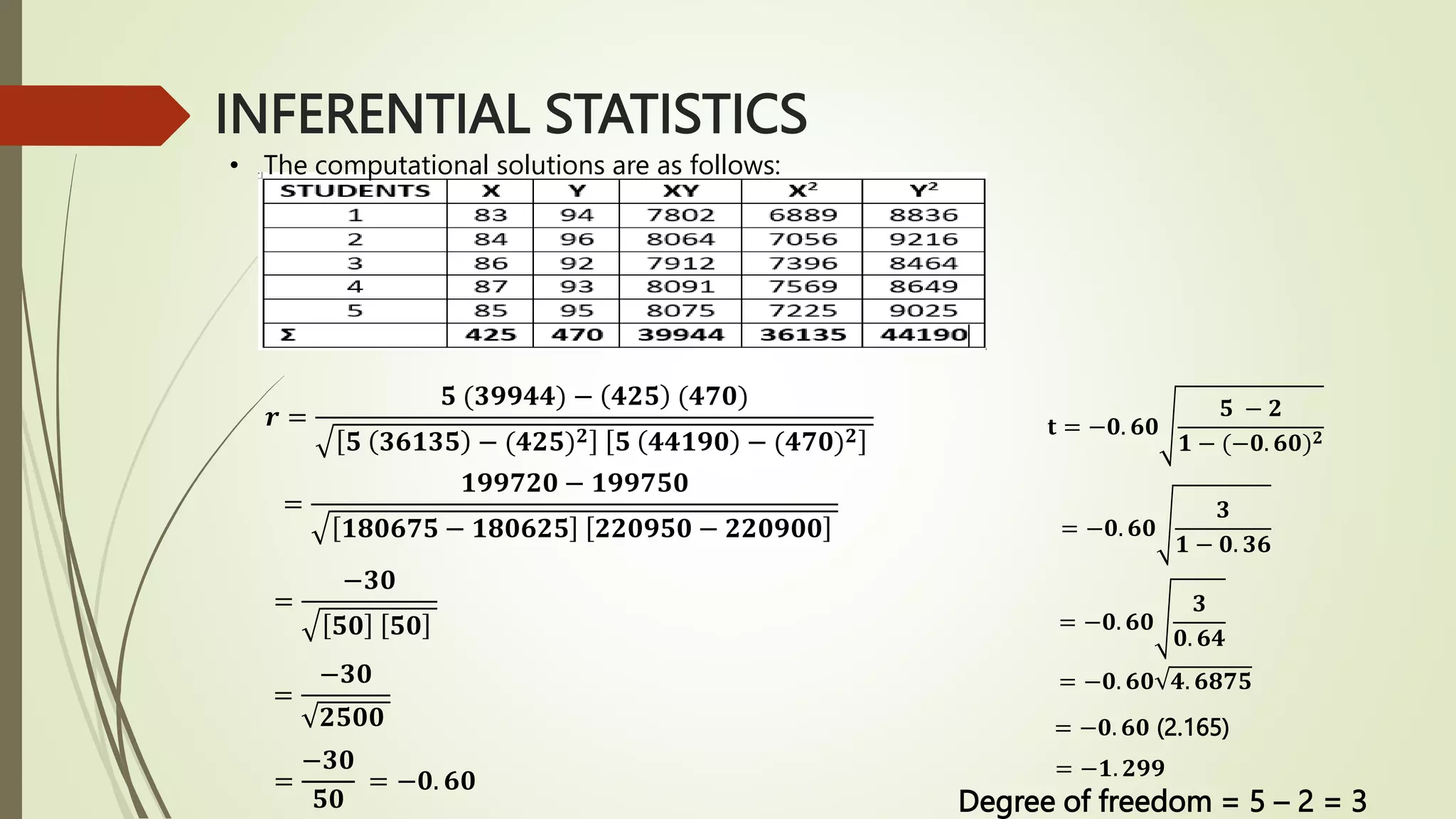
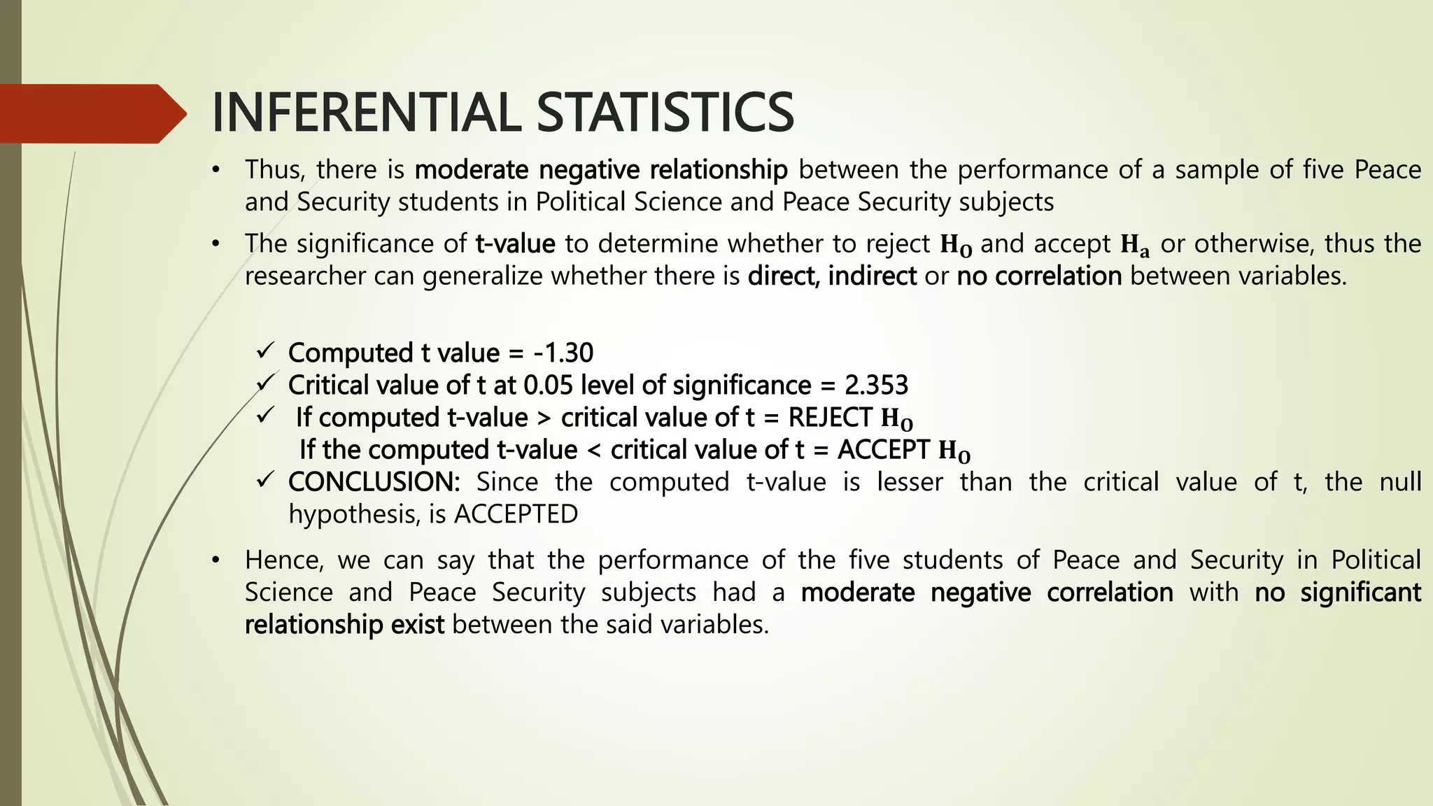
SlideShare a Scribd company logo
ADVANCE STATISTICS
Jemer M. Mabazza, LLB, PhD
Graduate School
Mallig Plains Colleges
INFERENTIAL STATISTICS
 Inferential Statistics
• Refers to the statistical procedure used in the drawing of inferences about the
properties of population from sample data.
 Test of Hypothesis
• It is a statistical tool that determines whether there is a statistically significant
difference between two or more groups, or whether there is a statistically significant
relationship between two or more variables.
 Hypothesis
• It is a statement or tentative theory which aims to explain a facts about the real world.
• They are subjected to testing.
 If they are found to be statistically true, they are accepted
 If they are found to be statistically false, they are rejected
INFERENTIAL STATISTICS
 Two Kinds of Hypothesis
1. Null Hypothesis (H0). A hypothesis that may either be rejected or accepted
2. Alternative Hypothesis (Ha). It generally represents the hypothetical statement the
that the researcher wanted to prove.
• Summary:
 REJECTION of H0 implies ACCEPTANCE of Ha
 ACCEPTANCE of H0 implies REJECTION of Ha
• Possible Error when Making Decision about the Proposed Hypothesis- SUMMARY:
TYPE I and TYPE II ERRORS
DECISION H0 = TRUE Actual Condition
Ha = TRUE
Reject H0 Type I Error Correct Decision
Accept H0 Correct Decision Type II Error
• The probability of making a type 1 error or alpha error in a test is called a significance
level of a test.
INFERENTIAL STATISTICS
 Steps in Hypothesis Testing
1. Formulate the null hypothesis (H0) that there is no significant difference between
items being compared.
2. Set the level of significance.
3. Determine the test to be used.
4. Determine the tabular value for the test.
5. Compute for z-test or t-test as needed.
 z – test
1. Sample mean compared with Population mean
FORMULA:
z =
X − µ
σ
𝑛
where: z = z-test
X = sample mean
µ = population mean
σ = population standard deviation
n = number of items within the sample
INFERENTIAL STATISTICS
2. Comparing two sample mean
FORMULA: Z =
X1 − X2
σ 1
n1
+
1
n2
where: z = z-test
X1 = mean of the first sample
X2 = mean of the second sample
n1 = number of items in the second sample
σ = population standard deviation
3. Comparing two sample proportions
FORMULA:
where: P1 = proportion of the first sample
q1 = 1 - P1
P2 = proportion of second sample
q2 = 1 - P2
n1 = number of items in the first sample
n2 = number of items in the second sample
𝑧 =
P1 −
P2
P1q1
n1
+
P2q2
n2
INFERENTIAL STATISTICS
 EXAMPLE 1
Data from a school census show that the mean weight of college students was 45 kilos,
with a standard deviation of 3 kilos. A sample of 100 college students were found to have
a mean weight of 47 kilos. Are the 100 college students really heavier than the rest, using
.05 significance level?
Step 1: H0 : The 100 college students are not really heavier that the rest. (X = 45 kilos)
Ha : The 100 college students are really heavier that the rest. (X > 45 kilos)
Step 2: Set 0.05 level of significance
Step 3: The standard deviation given is based on the population. Therefore the z-test is to be
used
Step 4: Based on the table (critical value of z), the tabular value of z for one tailed test at 0.05
level of significance is 1.645
Step 5: The given values in the problem are:
X = 47 kilos
µ = 45 kilos
σ = 3 kilos
n = 100
INFERENTIAL STATISTICS
FORMULA: z =
X − µ
σ
𝑛
z =
47 −45
3
100
=
2
3
10
=
2
0.3
= 6.67
Step 6: The computed value of 6.67 is greater than the tabular value 1.645. Therefore, the null
hypothesis is rejected
INFERENTIAL STATISTICS
 EXAMPLE 2
A researcher wishes to find out whether or not there is significant difference between the
monthly allowance of morning and afternoon students In his school. By random
sampling, he took a sample of 239 students in the morning session. These students were
found to have a mean of monthly allowance of ₱142.00. The researcher also took a
sample of 209 students in the afternoon session. They were found to have a mean
monthly allowance of ₱148.00. The total population of students in that school has a
standard deviation of ₱40. Is there a significant difference between the two samples at
0.01 level of significance?
H0 : There is no significant difference between the samples
Ha : There is significant difference between the samples
FORMULA: Z =
X1 − X2
σ 1
n1
+
1
n2
INFERENTIAL STATISTICS
Z =
142 −148
40 1
239
+
1
209
=
−6
40
0.0042 +0.0048
=
−6
40
0.0090
=
−6
40 (0.095)
=
−6
3.8
= −1.579
The computed value of 1.579 is less than the tabular value of 2.58 at 0.01 level of significance.
Accept the null hypothesis
INFERENTIAL STATISTICS
 EXAMPLE 3
A sample survey of a television program in Metro Manila shows that 80 of 200 men
dislike the same program. We want to decide whether the difference between the two
sample proportion,
80
200
= 0.40 and
75
250
= 0.30, is significant or not at 0.05 level of
significance.
H0 : There is no significant difference between the two sample proportions
Ha : There is significant difference between the two sample proportions
The given values in the problem are:
P1 = 0.40 q1 = 1 - P1 = 1 – 0.40 = 0.60
P2 = 0.30 q2 = 1 - P2 = 1 – 0.30 = 0.70
n1 = 200 n2 = 250
𝑧 =
P1 −
P2
P1q1
n1
+
P2q2
n2
𝑧 =
0.40 − 0.30
(0.40) (0.60)
200
+
(0.30) 0.70)
250
=
0.10
0.24
200
+
0.21
250
=
0.10
0.0012 + 0.00084
INFERENTIAL STATISTICS
=
0.10
0.00204
=
0.10
0.045
= 2.22
The computed value of 2.22 is greater than the tabular value 1.96, the null hypothesis is
rejected
INFERENTIAL STATISTICS
 t – test
1. Sample mean compared with Population mean
FORMULA: t =
X − µ
𝑠
𝑛 −1
or t =
X − µ 𝑛 −1
𝑠
where: t = t-test
X = sample mean
µ = population mean
s = sample standard deviation
n = number of items in the sample
EXAMPLE: A researchers knows that the average height of Filipino women is 1.525
meters. A random sample of 26 women was taken and was found to have a mean
height of 1.56 , with standard deviation of .10 meters. Is there reason to believe that
the 26 women in the sample are significantly taller than the others .05 significance
level?
H0 : The sample is not significantly taller than the other Filipino women
Ha : The sample is significantly taller than the others
INFERENTIAL STATISTICS
The given values in the problem are:
X = 1.56 meters
µ = 1.525 meters
s = .10 meters
n = 26
degrees of freedom = n – 1
= 26 – 1
= 25
FORMULA: t =
X − µ
𝑠
𝑛 −1
t =
1.56 −1.525
.10
26 −1
t =
0.035
.10
25
t =
0.035
0.02
t = 1.75
The computed value of 1.75 is greater than the tabular value 1.708, the null hypothesis is
rejected
INFERENTIAL STATISTICS
2. Comparing two sample means
FORMULA: t =
X1 − X2
(𝑛1−1) 𝑠1
2+(𝑛2−1) 𝑠2
2
𝑛1+ 𝑛2 −2
1
𝑛1
+
1
𝑛2
where: t = t-test
X1 = mean of the first sample
X2 = mean of the second sample
𝑠1 = standard deviation of the first sample
𝑠2 = standard deviation of the second sample
𝑛1 = number of items in the first sample
𝑛2 = number of items in the second sample
INFERENTIAL STATISTICS
EXAMPLE: A teacher wishes to test whether or not the Case Method of teaching is more effective that
the Traditional Method. She picks two classes of approximately equal intelligence (verified trough an
administered IQ test). She gathers a sample of 18 students to whom she uses the Case Method and
another sample of 14 students to whom she uses the Traditional Method. After the experiment, an
objective tests revealed that the first sample got a mean score of 28.6 with a standard deviation of 5.9,
while the second group got a mean score of 21.7 with a standard deviation of 4.6. Based on the result
of the administered test, can we say that the Case Method is more effective that the Traditional
Method?
H0 : The Case Method is as effective as the Traditional Method
Ha : The Case Method is more effective that the Traditional Method
Given:X1 = 28.6 X2 = 21.7
𝑠1 = 5.9 𝑠2 = 4.6
𝑛1 = 18 𝑛2 = 14
degrees of freedom = 𝑛1 + 𝑛2 - 2
= 18 + 14 – 2
= 30
INFERENTIAL STATISTICS
FORMULA: t =
X1 − X2
(𝑛1−1) 𝑠1
2+(𝑛2−1) 𝑠2
2
𝑛1+ 𝑛2 −2
1
𝑛1
+
1
𝑛2
t =
28.6 −21.7
18−1 5.9 2+(14−1) 4.6 2
18 +14 −2
1
18
+
1
14
t =
6.9
17 (34.81)+(13) (21.16)
32 −2
0.06+0.07
t =
6.9
591.77+275.08
30
0.13
t =
6.9
28.895 0.13
t =
6.9
3.756
t =
6.9
1.94
t =3.56
The computed t-value of 3.56 is greater than the tabular value 1.697, therefore the null
hypothesis is rejected
INFERENTIAL STATISTICS
 Analysis of Variance (ANOVA)
FORMULA:
F =
MSS𝑏
MSS𝑤
• ANOVA is based upon two sources of variation – (1) the between – column variance;
(2) the within – column variance
• The two variance was sometimes called as between – column sum of squares (𝐒𝐒𝒃)
and the within – column sum of squares (𝑺𝑺𝑤). The sum of the two variances make up
the total sum of squares (TSS).
FORMULA: TSS = 𝑥2 −
( 𝑥)2
𝑁
where: x = refers to the value of each entry
N = refers to the total number of items
EXAMPLE: Let us take three groups of 6 students each, where each group is subjected to
one of three types of teaching method. The grades of the students are taken at the end
of the semester and enumerated according to grouping. The one way classification
model will look like this:
INFERENTIAL STATISTICS
Group I
Method A
Group II
Method B
Group III
Method C
Student 1
Student 2
Student 3
Student 4
Student 5
Student 6
84
90
92
96
84
88
70
75
90
80
75
75
90
95
100
98
88
90
(𝑋𝑎)2 (𝑋𝑏)2
(𝑋𝑐)2
7,056
8,100
8,464
9,216
7,056
7,744
4,900
5,625
8,100
6,400
5,625
5,625
8,100
9,025
10,000
9,604
7,744
7,744
534 465 561 47,636 36,275 52,573
𝑋 = 534 + 465 + 561 = 1, 560
𝑋2 = 47, 636 + 36, 275 + 52, 573 = 𝟏𝟑𝟔, 𝟒𝟖𝟒
INFERENTIAL STATISTICS
• The total sum of squares is computed as follows:
TSS = 136, 484 -
(1,560)2
18
= 136, 484 -
2,433,600
18
= 136, 484 - 135, 200
= 1, 284
• The between-column variance or between-column sum of squares is of the sum of the squares
of the column sum, minus the correction term, where r refers to the number of rows.
1
𝑟
𝑆𝑆𝑏 =
1
𝑁𝑜. 𝑜𝑓 𝑅𝑜𝑤𝑠
(𝑠𝑢𝑚 𝑜𝑓 𝑒𝑎𝑐ℎ 𝑐𝑜𝑙𝑢𝑚𝑛)2
−
( 𝑥)
2
𝑁
𝑆𝑆𝑏 =
1
6
(5342
+ 4652
+ 5612
) −
(1, 560)2
18
𝑆𝑆𝑏 =
1
6
(285, 156 + 216, 255 + 314, 721) −
(2, 433, 600)
18
𝑆𝑆𝑏 =
816, 132
6
−
(2, 433, 600)
18
𝑆𝑆𝑏 = 136, 022 − 135, 200
𝑆𝑆𝑏 = 822
TSS = 𝑥2
−
( 𝑥)2
𝑁
INFERENTIAL STATISTICS
• The within-column variance or within-column sum of squares is the difference between the total
sum of squares and the between-column sum of squares.
𝑆𝑆𝑤 = TSS − SS𝑏
= 1, 284 − 822
= 462
• We can make use any of the following in getting the “degrees of freedom”:
Total degress of freedom (df) = N − 1
= 18 − 1
= 𝟏𝟕
Total degress of freedom (df) = rk − 1
= (3 x 6) − 1
= 18 − 1
= 𝟏𝟕
Between-column df = Number of Columns – 1
= 3 − 1
= 𝟐
Within-column df = total df – between column df
= 17 − 2
= 𝟏𝟓
INFERENTIAL STATISTICS
• To compute for the Mean Sum of Squares
𝑀𝑆𝑆𝑏 =
SS𝑏
df𝑏
=
822
2
= 411
𝑀𝑆𝑆𝑤 =
SS𝑤
df𝑤
=
462
15
= 30.8
• To compute for the F-test
F =
MSS𝑏
MSS𝑤
F =
411
30.8
= 13.34
INFERENTIAL STATISTICS
• ANOVA Table on the Three Samples Subjected to Different Teaching Method
• The tabular value: 3.68 at 5% level of significance
• DECISION: The null hypothesis is rejected considering that the computed value of 13.34 is greater
than the tabular value of 3.68
INFERENTIAL STATISTICS
 Chi-square Test (𝑿𝟐
)
• Use of Chi-square Test
1. For estimating how closely an observed distribution matches an expected
distribution, also known as good-of-fit test.
2. For estimating whether two random variables are independent, also called as test
of independence.
FORMULA: For Good-of-Fit Test
𝑋2
=
(OF − EF)2
EF
FORMULA: For Test of Independence
𝑋2
=
(OF − EF)2
EF
EF =
Row Total x Column Total
n
INFERENTIAL STATISTICS
 EXAMPLE
• Chi-square for a Good-of-Fit Test
 A two dice (dice A and B) with six sides was rolled out 10 times with a chance of any
particular number coming out was the same: 1 in 6. If the dice is loaded, there are certain
numbers which will have a greater chance of appearing, while others will have a lower
chance. The researcher observed the following in one dice (A).
𝑥2
=
(18−10)2
10
+
(5−10)2
10
+
(9−10)2
10
+
(7−10)2
10
+
(5−10)2
10
+
(16−10)2
10
𝑥2 = 6.4 + 2.5 + 0.1 + 0.9 + 2.5 + 3.6
𝑥2 = 16 CONCLUSION: There is very low chance that these rolls came from a fair dice considering that the calculated
value of 16 is greater that the tabular value of 11.07. This means that there is statistically significant difference
between the two dices.
INFERENTIAL STATISTICS
• Chi-square Test for Independence
• Test the hypothesis that academic performance does not depend on IQ at 1% significance level.
• Degrees of Freedom (df) = (r – 1) (k – 1)
= (2 – 1) (3 – 1)
= 2
• COMPUTATION: Getting the 𝐅𝒆
 Where 𝑓𝑜 = 31, 𝑓𝑒 =
32 x 80
100
= 25.6
 Where 𝑓𝑜 = 1, 𝑓𝑒 =
32 x 20
100
= 6.4
 Where 𝑓𝑜 = 45, 𝑓𝑒 =
49 x 80
100
= 39.20
 Where 𝑓𝑜 = 4, 𝑓𝑒 =
49 x 20
100
= 9.80
 Where 𝑓𝑜 = 4, 𝑓𝑒 =
19 x 80
100
= 15.2
 Where 𝑓𝑜 = 15, 𝑓𝑒 =
19 x 20
100
= 3.80
INFERENTIAL STATISTICS
• Replacing the above values into the chi-square formula, we shall have:
𝑋2 =
(OF − EF)2
EF
𝑋2
=
(31 −25.6)2
25.6
+
(1 −6.4)2
6.4
+
(45 −39.2)2
39.2
+
(4 −9.80)2
9.80
+
(4 −15.2)2
15.2
+
(15 −3.80)2
3.80
𝑋2 =
29.16
25.6
+
29.16
6.4
+
33.64
39.2
+
33.64
9.80
+
125.44
15.2
+
125.44
3.80
𝑋2 = 1.139 + 4.556 + 0.858 + 3.433 + 8.253 + 33.011
𝑋2 = 51.25
• Since the computed Chi-square value of 51.25 is greater than the tabular value of 9.21, the null
hypothesis is rejected. For the 100 students, academic performance depends on IQ
INFERENTIAL STATISTICS
 Simple Regression Analysis
• Regression analysis is concerned with the problem of estimation and forecasting.
 TYPES OF RELATIONSHIP
1. Direct Relationship. The slope of the line is positive because Y increases as X also
increases
2. Inverse Relationship. The slope of the line is negative because Y decreases as X also
increases
• Least Square Regression Line or LSRL is a statistical technique that analyses the
relationship between the independent and dependent variables.
 EQUATION:
Y = a + bX
 NORMAL EQUATIONS:
1. ΣY = aN + bΣX
2. ΣXY = aΣX + bΣ𝑿𝟐
INFERENTIAL STATISTICS
WHERE: ΣY = sum of the values of Y, the dependent variable
N = the number of pairs of X and Y
ΣX = sum of the values of X, the independent variable
ΣXY = the sum of the column XY, which is derived by multiplying the paired values of X and Y
Σ𝐗𝟐
= the sum of the column 𝐗𝟐
is derived by squaring the values of X
• Based on the given data of X and Y, we can determine all of the above which means
that the two normal equations now consist of a system of two linear equations with
two unknowns – a and b
• FORMULAS:
a=
𝚺𝐘 𝚺𝐗𝟐 − 𝚺𝐗 (𝜮𝑿𝒀)
𝐍 𝜮𝐗𝟐 −(𝜮𝐗)𝟐
b=
𝐍 𝜮𝐗𝐘 − 𝜮𝐗 (𝜮𝐘)
𝐍 𝜮𝐗𝟐 − (𝜮𝐗)𝟐
INFERENTIAL STATISTICS
• EXAMPLE:
X Y XY X2
1
3
4
6
8
9
11
14
56
1
2
4
4
5
7
8
8
40
1
6
16
24
40
63
88
126
1
9
16
36
64
81
121
196
364 524
a=
40 524 − 56 (364)
8 524 −(56)2
a=
20960−20384
4192 −3136
a=
576
1056
= 𝟎. 𝟓𝟒
b=
8 364 − 56 (40)
8 524 − (56)2
b=
2912−2240
4192 −3136
b=
672
1056
= 𝟎. 𝟔𝟒
Y = 0.54 + 0.64 (16)
= 0.54 + 10.24
= 10.78
INFERENTIAL STATISTICS
 Simple Correlation Analysis
• Correlation analysis concerned with the relationship in the changes of such variables.
• Degrees of correlation or relationship between two variables
1. Perfect correlation (negative and positive)
2. Some degrees of correlation (negative and positive)
3. No correlation
• The concept of correlation in terms of computed value is called correlation coefficient.
The value of the correlation coefficient ranges from -1 to +1.
• Pearson r test. The Pearson Product-Moment Coefficient of Correlation, otherwise
known as Pearson r is the most commonly used correlation coefficient.
• Pearson r, as the most widely used measure of correlation has two basic assumptions,
to wit:
1. The existence of linear relationship; and
2. The level of measurement of the data for the two variables are either in interval or
ratio scale.
INFERENTIAL STATISTICS
• The value of r (degree of linear relationship) can be interpreted according to the use of
range of values for the Pearson Product Moment of Correlation Coefficient, as follows:
• Notably, Pearson r is not a measure of causality. The significant of the obtained
correlation coefficient can be determined through the use of t-test for testing the
significance of r.
𝐭 = 𝐫
𝐧 − 𝟐
𝟏 − 𝐫𝟐
WHERE: t = t-test
r = obtained Pearson r value
n = paired sample size
FORMULA:
Degree of freedom = n – 2
INFERENTIAL STATISTICS
FORMULA for Pearson r:
𝒓 =
𝐍 𝚺𝐗𝐘 − 𝚺𝐗 (𝚺𝐘)
𝐍 𝜮𝐗𝟐 − (𝜮𝐗)𝟐 𝐍 𝜮𝐘𝟐 − (𝜮𝐘)𝟐
Where: r = correlation coefficient
N = total number of pair variables
X = the first variable under study
Y = the second variable under study
EXAMPLE:
A researcher wants to find out about the relationship between the performance of a sample
of five Peace and Security students in Political Science and Peace Security subjects:
INFERENTIAL STATISTICS
• The computational solutions are as follows:
𝒓 =
𝟓 (𝟑𝟗𝟗𝟒𝟒) − 𝟒𝟐𝟓 (𝟒𝟕𝟎)
𝟓 𝟑𝟔𝟏𝟑𝟓 − (𝟒𝟐𝟓)𝟐 𝟓 𝟒𝟒𝟏𝟗𝟎 − (𝟒𝟕𝟎)𝟐
=
𝟏𝟗𝟗𝟕𝟐𝟎 − 𝟏𝟗𝟗𝟕𝟓𝟎
𝟏𝟖𝟎𝟔𝟕𝟓 − 𝟏𝟖𝟎𝟔𝟐𝟓 𝟐𝟐𝟎𝟗𝟓𝟎 − 𝟐𝟐𝟎𝟗𝟎𝟎
=
−𝟑𝟎
𝟓𝟎 𝟓𝟎
=
−𝟑𝟎
𝟐𝟓𝟎𝟎
=
−𝟑𝟎
𝟓𝟎
= −𝟎. 𝟔𝟎
𝐭 = −𝟎. 𝟔𝟎
𝟓 − 𝟐
𝟏 − (−𝟎. 𝟔𝟎)𝟐
= −𝟎. 𝟔𝟎
𝟑
𝟏 − 𝟎. 𝟑𝟔
= −𝟎. 𝟔𝟎
𝟑
𝟎. 𝟔𝟒
= −𝟎. 𝟔𝟎 𝟒. 𝟔𝟖𝟕𝟓
= −𝟎. 𝟔𝟎 (2.165)
= −𝟏. 𝟐𝟗𝟗
Degree of freedom = 5 – 2 = 3
INFERENTIAL STATISTICS
• Thus, there is moderate negative relationship between the performance of a sample of five Peace
and Security students in Political Science and Peace Security subjects
• The significance of t-value to determine whether to reject 𝐇𝐎 and accept 𝐇𝐚 or otherwise, thus the
researcher can generalize whether there is direct, indirect or no correlation between variables.
 Computed t value = -1.30
 Critical value of t at 0.05 level of significance = 2.353
 If computed t-value > critical value of t = REJECT 𝐇𝐎
If the computed t-value < critical value of t = ACCEPT 𝐇𝐎
 CONCLUSION: Since the computed t-value is lesser than the critical value of t, the null
hypothesis, is ACCEPTED
• Hence, we can say that the performance of the five students of Peace and Security in Political
Science and Peace Security subjects had a moderate negative correlation with no significant
relationship exist between the said variables.

More Related Content

What's hot

Measures of variability
Measures of variabilityMeasures of variability
Measures of variability
jennytuazon01630
 
The Standard Normal Distribution
The Standard Normal Distribution  The Standard Normal Distribution
The Standard Normal Distribution
Long Beach City College
 
Writing up your results – apa style guidelines
Writing up your results – apa style guidelinesWriting up your results – apa style guidelines
Writing up your results – apa style guidelines
Marialena Kostouli
 
Normal Curve
Normal CurveNormal Curve
Normal Curve
Ace Matilac
 
6. point and interval estimation
6. point and interval estimation6. point and interval estimation
6. point and interval estimation
ONE Virtual Services
 
QUARTILES, DECILES AND PERCENTILES
QUARTILES, DECILES  AND PERCENTILESQUARTILES, DECILES  AND PERCENTILES
QUARTILES, DECILES AND PERCENTILES
MARIA KATRINA MACAPAZ
 
Statistics "Descriptive & Inferential"
Statistics "Descriptive & Inferential"Statistics "Descriptive & Inferential"
Statistics "Descriptive & Inferential"
Dalia El-Shafei
 
z-test
z-testz-test
Weighted Mean - Class Average
Weighted Mean - Class AverageWeighted Mean - Class Average
Weighted Mean - Class Average
ccooking
 
Determining measures of central tendency for grouped data
Determining measures of central tendency for grouped dataDetermining measures of central tendency for grouped data
Determining measures of central tendency for grouped data
Alona Hall
 
Data management through spss
Data management through spssData management through spss
Data management through spss
APPOLINAIRE BIZIMANA
 
numerical method in statistics (MEAN AND MEDIAN)
numerical method in statistics (MEAN AND MEDIAN)numerical method in statistics (MEAN AND MEDIAN)
numerical method in statistics (MEAN AND MEDIAN)
METRO MANILA COLLEGE
 
Non Parametric Statistics
Non Parametric StatisticsNon Parametric Statistics
Non Parametric Statistics
jennytuazon01630
 
4. parameter and statistic
4. parameter and statistic4. parameter and statistic
4. parameter and statistic
ONE Virtual Services
 
Measures of central tendency
Measures of central tendencyMeasures of central tendency
Measures of central tendency
Chie Pegollo
 
frequency distribution
 frequency distribution frequency distribution
frequency distribution
Unsa Shakir
 
Normal distribution and sampling distribution
Normal distribution and sampling distributionNormal distribution and sampling distribution
Normal distribution and sampling distribution
Mridul Arora
 
Systematic sampling in probability sampling
Systematic sampling in probability sampling Systematic sampling in probability sampling
Systematic sampling in probability sampling
Sachin H
 
Measures of variability grouped data
Measures of variability grouped dataMeasures of variability grouped data
Measures of variability grouped data
Jean Claudette Tolentino
 
parametric test of difference z test f test one-way_two-way_anova
parametric test of difference z test f test one-way_two-way_anova parametric test of difference z test f test one-way_two-way_anova
parametric test of difference z test f test one-way_two-way_anova
Tess Anoza
 

What's hot (20)

Measures of variability
Measures of variabilityMeasures of variability
Measures of variability
 
The Standard Normal Distribution
The Standard Normal Distribution  The Standard Normal Distribution
The Standard Normal Distribution
 
Writing up your results – apa style guidelines
Writing up your results – apa style guidelinesWriting up your results – apa style guidelines
Writing up your results – apa style guidelines
 
Normal Curve
Normal CurveNormal Curve
Normal Curve
 
6. point and interval estimation
6. point and interval estimation6. point and interval estimation
6. point and interval estimation
 
QUARTILES, DECILES AND PERCENTILES
QUARTILES, DECILES  AND PERCENTILESQUARTILES, DECILES  AND PERCENTILES
QUARTILES, DECILES AND PERCENTILES
 
Statistics "Descriptive & Inferential"
Statistics "Descriptive & Inferential"Statistics "Descriptive & Inferential"
Statistics "Descriptive & Inferential"
 
z-test
z-testz-test
z-test
 
Weighted Mean - Class Average
Weighted Mean - Class AverageWeighted Mean - Class Average
Weighted Mean - Class Average
 
Determining measures of central tendency for grouped data
Determining measures of central tendency for grouped dataDetermining measures of central tendency for grouped data
Determining measures of central tendency for grouped data
 
Data management through spss
Data management through spssData management through spss
Data management through spss
 
numerical method in statistics (MEAN AND MEDIAN)
numerical method in statistics (MEAN AND MEDIAN)numerical method in statistics (MEAN AND MEDIAN)
numerical method in statistics (MEAN AND MEDIAN)
 
Non Parametric Statistics
Non Parametric StatisticsNon Parametric Statistics
Non Parametric Statistics
 
4. parameter and statistic
4. parameter and statistic4. parameter and statistic
4. parameter and statistic
 
Measures of central tendency
Measures of central tendencyMeasures of central tendency
Measures of central tendency
 
frequency distribution
 frequency distribution frequency distribution
frequency distribution
 
Normal distribution and sampling distribution
Normal distribution and sampling distributionNormal distribution and sampling distribution
Normal distribution and sampling distribution
 
Systematic sampling in probability sampling
Systematic sampling in probability sampling Systematic sampling in probability sampling
Systematic sampling in probability sampling
 
Measures of variability grouped data
Measures of variability grouped dataMeasures of variability grouped data
Measures of variability grouped data
 
parametric test of difference z test f test one-way_two-way_anova
parametric test of difference z test f test one-way_two-way_anova parametric test of difference z test f test one-way_two-way_anova
parametric test of difference z test f test one-way_two-way_anova
 

Similar to INFERENTIAL STATISTICS.pptx

Statistical analysis.pptx
Statistical analysis.pptxStatistical analysis.pptx
Statistical analysis.pptx
Chinna Chadayan
 
Analysis of variance (ANOVA)
Analysis of variance (ANOVA)Analysis of variance (ANOVA)
Analysis of variance (ANOVA)
Sneh Kumari
 
inferentialstatistics-210411214248.pdf
inferentialstatistics-210411214248.pdfinferentialstatistics-210411214248.pdf
inferentialstatistics-210411214248.pdf
ChenPalaruan
 
Inferential statistics
Inferential statisticsInferential statistics
Inferential statistics
Dalia El-Shafei
 
Lecture 11 Paired t test.pptx
Lecture 11 Paired t test.pptxLecture 11 Paired t test.pptx
Lecture 11 Paired t test.pptx
shakirRahman10
 
Chapter 7Hypothesis Testing ProceduresLearning.docx
Chapter 7Hypothesis Testing ProceduresLearning.docxChapter 7Hypothesis Testing ProceduresLearning.docx
Chapter 7Hypothesis Testing ProceduresLearning.docx
mccormicknadine86
 
Non parametrics tests
Non parametrics testsNon parametrics tests
Non parametrics tests
rodrick koome
 
Statistical analysis
Statistical  analysisStatistical  analysis
Statistical analysis
Princy Francis M
 
Test of significance
Test of significanceTest of significance
Test of significance
Dr. Imran Zaheer
 
Sampling distribution.pptx
Sampling distribution.pptxSampling distribution.pptx
Sampling distribution.pptx
ssusera0e0e9
 
Statistical analysis by iswar
Statistical analysis by iswarStatistical analysis by iswar
Central Tendency & Dispersion
Central Tendency & DispersionCentral Tendency & Dispersion
Central Tendency & Dispersion
Birinder Singh Gulati
 
Parametric tests
Parametric testsParametric tests
Parametric tests
Ananya Sree Katta
 
Str t-test1
Str   t-test1Str   t-test1
Str t-test1
iamkim
 
Testing hypothesis (methods of testing the statement of organizations)
Testing hypothesis (methods of testing the statement of organizations)Testing hypothesis (methods of testing the statement of organizations)
Testing hypothesis (methods of testing the statement of organizations)
syedahadisa929
 
NON-PARAMETRIC TESTS.pptx
NON-PARAMETRIC TESTS.pptxNON-PARAMETRIC TESTS.pptx
NON-PARAMETRIC TESTS.pptx
DrLasya
 
In a left-tailed test comparing two means with variances unknown b.docx
In a left-tailed test comparing two means with variances unknown b.docxIn a left-tailed test comparing two means with variances unknown b.docx
In a left-tailed test comparing two means with variances unknown b.docx
bradburgess22840
 
UNIT 5.pdf
UNIT 5.pdfUNIT 5.pdf
UNIT 5.pdf
RajaRokkala
 
Hypothesis_testing,regarding software engineering
Hypothesis_testing,regarding software engineeringHypothesis_testing,regarding software engineering
Hypothesis_testing,regarding software engineering
TallapelliSharanya01
 
Test of significance in Statistics
Test of significance in StatisticsTest of significance in Statistics
Test of significance in Statistics
Vikash Keshri
 

Similar to INFERENTIAL STATISTICS.pptx (20)

Statistical analysis.pptx
Statistical analysis.pptxStatistical analysis.pptx
Statistical analysis.pptx
 
Analysis of variance (ANOVA)
Analysis of variance (ANOVA)Analysis of variance (ANOVA)
Analysis of variance (ANOVA)
 
inferentialstatistics-210411214248.pdf
inferentialstatistics-210411214248.pdfinferentialstatistics-210411214248.pdf
inferentialstatistics-210411214248.pdf
 
Inferential statistics
Inferential statisticsInferential statistics
Inferential statistics
 
Lecture 11 Paired t test.pptx
Lecture 11 Paired t test.pptxLecture 11 Paired t test.pptx
Lecture 11 Paired t test.pptx
 
Chapter 7Hypothesis Testing ProceduresLearning.docx
Chapter 7Hypothesis Testing ProceduresLearning.docxChapter 7Hypothesis Testing ProceduresLearning.docx
Chapter 7Hypothesis Testing ProceduresLearning.docx
 
Non parametrics tests
Non parametrics testsNon parametrics tests
Non parametrics tests
 
Statistical analysis
Statistical  analysisStatistical  analysis
Statistical analysis
 
Test of significance
Test of significanceTest of significance
Test of significance
 
Sampling distribution.pptx
Sampling distribution.pptxSampling distribution.pptx
Sampling distribution.pptx
 
Statistical analysis by iswar
Statistical analysis by iswarStatistical analysis by iswar
Statistical analysis by iswar
 
Central Tendency & Dispersion
Central Tendency & DispersionCentral Tendency & Dispersion
Central Tendency & Dispersion
 
Parametric tests
Parametric testsParametric tests
Parametric tests
 
Str t-test1
Str   t-test1Str   t-test1
Str t-test1
 
Testing hypothesis (methods of testing the statement of organizations)
Testing hypothesis (methods of testing the statement of organizations)Testing hypothesis (methods of testing the statement of organizations)
Testing hypothesis (methods of testing the statement of organizations)
 
NON-PARAMETRIC TESTS.pptx
NON-PARAMETRIC TESTS.pptxNON-PARAMETRIC TESTS.pptx
NON-PARAMETRIC TESTS.pptx
 
In a left-tailed test comparing two means with variances unknown b.docx
In a left-tailed test comparing two means with variances unknown b.docxIn a left-tailed test comparing two means with variances unknown b.docx
In a left-tailed test comparing two means with variances unknown b.docx
 
UNIT 5.pdf
UNIT 5.pdfUNIT 5.pdf
UNIT 5.pdf
 
Hypothesis_testing,regarding software engineering
Hypothesis_testing,regarding software engineeringHypothesis_testing,regarding software engineering
Hypothesis_testing,regarding software engineering
 
Test of significance in Statistics
Test of significance in StatisticsTest of significance in Statistics
Test of significance in Statistics
 

Recently uploaded

一比一原版(UCSB文凭证书)圣芭芭拉分校毕业证如何办理
一比一原版(UCSB文凭证书)圣芭芭拉分校毕业证如何办理一比一原版(UCSB文凭证书)圣芭芭拉分校毕业证如何办理
一比一原版(UCSB文凭证书)圣芭芭拉分校毕业证如何办理
nuttdpt
 
The Building Blocks of QuestDB, a Time Series Database
The Building Blocks of QuestDB, a Time Series DatabaseThe Building Blocks of QuestDB, a Time Series Database
The Building Blocks of QuestDB, a Time Series Database
javier ramirez
 
DSSML24_tspann_CodelessGenerativeAIPipelines
DSSML24_tspann_CodelessGenerativeAIPipelinesDSSML24_tspann_CodelessGenerativeAIPipelines
DSSML24_tspann_CodelessGenerativeAIPipelines
Timothy Spann
 
Intelligence supported media monitoring in veterinary medicine
Intelligence supported media monitoring in veterinary medicineIntelligence supported media monitoring in veterinary medicine
Intelligence supported media monitoring in veterinary medicine
AndrzejJarynowski
 
一比一原版(UMN文凭证书)明尼苏达大学毕业证如何办理
一比一原版(UMN文凭证书)明尼苏达大学毕业证如何办理一比一原版(UMN文凭证书)明尼苏达大学毕业证如何办理
一比一原版(UMN文凭证书)明尼苏达大学毕业证如何办理
nyfuhyz
 
06-12-2024-BudapestDataForum-BuildingReal-timePipelineswithFLaNK AIM
06-12-2024-BudapestDataForum-BuildingReal-timePipelineswithFLaNK AIM06-12-2024-BudapestDataForum-BuildingReal-timePipelineswithFLaNK AIM
06-12-2024-BudapestDataForum-BuildingReal-timePipelineswithFLaNK AIM
Timothy Spann
 
Beyond the Basics of A/B Tests: Highly Innovative Experimentation Tactics You...
Beyond the Basics of A/B Tests: Highly Innovative Experimentation Tactics You...Beyond the Basics of A/B Tests: Highly Innovative Experimentation Tactics You...
Beyond the Basics of A/B Tests: Highly Innovative Experimentation Tactics You...
Aggregage
 
Analysis insight about a Flyball dog competition team's performance
Analysis insight about a Flyball dog competition team's performanceAnalysis insight about a Flyball dog competition team's performance
Analysis insight about a Flyball dog competition team's performance
roli9797
 
Population Growth in Bataan: The effects of population growth around rural pl...
Population Growth in Bataan: The effects of population growth around rural pl...Population Growth in Bataan: The effects of population growth around rural pl...
Population Growth in Bataan: The effects of population growth around rural pl...
Bill641377
 
Learn SQL from basic queries to Advance queries
Learn SQL from basic queries to Advance queriesLearn SQL from basic queries to Advance queries
Learn SQL from basic queries to Advance queries
manishkhaire30
 
End-to-end pipeline agility - Berlin Buzzwords 2024
End-to-end pipeline agility - Berlin Buzzwords 2024End-to-end pipeline agility - Berlin Buzzwords 2024
End-to-end pipeline agility - Berlin Buzzwords 2024
Lars Albertsson
 
原版制作(unimelb毕业证书)墨尔本大学毕业证Offer一模一样
原版制作(unimelb毕业证书)墨尔本大学毕业证Offer一模一样原版制作(unimelb毕业证书)墨尔本大学毕业证Offer一模一样
原版制作(unimelb毕业证书)墨尔本大学毕业证Offer一模一样
ihavuls
 
Experts live - Improving user adoption with AI
Experts live - Improving user adoption with AIExperts live - Improving user adoption with AI
Experts live - Improving user adoption with AI
jitskeb
 
一比一原版(UCSF文凭证书)旧金山分校毕业证如何办理
一比一原版(UCSF文凭证书)旧金山分校毕业证如何办理一比一原版(UCSF文凭证书)旧金山分校毕业证如何办理
一比一原版(UCSF文凭证书)旧金山分校毕业证如何办理
nuttdpt
 
4th Modern Marketing Reckoner by MMA Global India & Group M: 60+ experts on W...
4th Modern Marketing Reckoner by MMA Global India & Group M: 60+ experts on W...4th Modern Marketing Reckoner by MMA Global India & Group M: 60+ experts on W...
4th Modern Marketing Reckoner by MMA Global India & Group M: 60+ experts on W...
Social Samosa
 
在线办理(英国UCA毕业证书)创意艺术大学毕业证在读证明一模一样
在线办理(英国UCA毕业证书)创意艺术大学毕业证在读证明一模一样在线办理(英国UCA毕业证书)创意艺术大学毕业证在读证明一模一样
在线办理(英国UCA毕业证书)创意艺术大学毕业证在读证明一模一样
v7oacc3l
 
Everything you wanted to know about LIHTC
Everything you wanted to know about LIHTCEverything you wanted to know about LIHTC
Everything you wanted to know about LIHTC
Roger Valdez
 
The Ipsos - AI - Monitor 2024 Report.pdf
The  Ipsos - AI - Monitor 2024 Report.pdfThe  Ipsos - AI - Monitor 2024 Report.pdf
The Ipsos - AI - Monitor 2024 Report.pdf
Social Samosa
 
Palo Alto Cortex XDR presentation .......
Palo Alto Cortex XDR presentation .......Palo Alto Cortex XDR presentation .......
Palo Alto Cortex XDR presentation .......
Sachin Paul
 
Open Source Contributions to Postgres: The Basics POSETTE 2024
Open Source Contributions to Postgres: The Basics POSETTE 2024Open Source Contributions to Postgres: The Basics POSETTE 2024
Open Source Contributions to Postgres: The Basics POSETTE 2024
ElizabethGarrettChri
 

Recently uploaded (20)

一比一原版(UCSB文凭证书)圣芭芭拉分校毕业证如何办理
一比一原版(UCSB文凭证书)圣芭芭拉分校毕业证如何办理一比一原版(UCSB文凭证书)圣芭芭拉分校毕业证如何办理
一比一原版(UCSB文凭证书)圣芭芭拉分校毕业证如何办理
 
The Building Blocks of QuestDB, a Time Series Database
The Building Blocks of QuestDB, a Time Series DatabaseThe Building Blocks of QuestDB, a Time Series Database
The Building Blocks of QuestDB, a Time Series Database
 
DSSML24_tspann_CodelessGenerativeAIPipelines
DSSML24_tspann_CodelessGenerativeAIPipelinesDSSML24_tspann_CodelessGenerativeAIPipelines
DSSML24_tspann_CodelessGenerativeAIPipelines
 
Intelligence supported media monitoring in veterinary medicine
Intelligence supported media monitoring in veterinary medicineIntelligence supported media monitoring in veterinary medicine
Intelligence supported media monitoring in veterinary medicine
 
一比一原版(UMN文凭证书)明尼苏达大学毕业证如何办理
一比一原版(UMN文凭证书)明尼苏达大学毕业证如何办理一比一原版(UMN文凭证书)明尼苏达大学毕业证如何办理
一比一原版(UMN文凭证书)明尼苏达大学毕业证如何办理
 
06-12-2024-BudapestDataForum-BuildingReal-timePipelineswithFLaNK AIM
06-12-2024-BudapestDataForum-BuildingReal-timePipelineswithFLaNK AIM06-12-2024-BudapestDataForum-BuildingReal-timePipelineswithFLaNK AIM
06-12-2024-BudapestDataForum-BuildingReal-timePipelineswithFLaNK AIM
 
Beyond the Basics of A/B Tests: Highly Innovative Experimentation Tactics You...
Beyond the Basics of A/B Tests: Highly Innovative Experimentation Tactics You...Beyond the Basics of A/B Tests: Highly Innovative Experimentation Tactics You...
Beyond the Basics of A/B Tests: Highly Innovative Experimentation Tactics You...
 
Analysis insight about a Flyball dog competition team's performance
Analysis insight about a Flyball dog competition team's performanceAnalysis insight about a Flyball dog competition team's performance
Analysis insight about a Flyball dog competition team's performance
 
Population Growth in Bataan: The effects of population growth around rural pl...
Population Growth in Bataan: The effects of population growth around rural pl...Population Growth in Bataan: The effects of population growth around rural pl...
Population Growth in Bataan: The effects of population growth around rural pl...
 
Learn SQL from basic queries to Advance queries
Learn SQL from basic queries to Advance queriesLearn SQL from basic queries to Advance queries
Learn SQL from basic queries to Advance queries
 
End-to-end pipeline agility - Berlin Buzzwords 2024
End-to-end pipeline agility - Berlin Buzzwords 2024End-to-end pipeline agility - Berlin Buzzwords 2024
End-to-end pipeline agility - Berlin Buzzwords 2024
 
原版制作(unimelb毕业证书)墨尔本大学毕业证Offer一模一样
原版制作(unimelb毕业证书)墨尔本大学毕业证Offer一模一样原版制作(unimelb毕业证书)墨尔本大学毕业证Offer一模一样
原版制作(unimelb毕业证书)墨尔本大学毕业证Offer一模一样
 
Experts live - Improving user adoption with AI
Experts live - Improving user adoption with AIExperts live - Improving user adoption with AI
Experts live - Improving user adoption with AI
 
一比一原版(UCSF文凭证书)旧金山分校毕业证如何办理
一比一原版(UCSF文凭证书)旧金山分校毕业证如何办理一比一原版(UCSF文凭证书)旧金山分校毕业证如何办理
一比一原版(UCSF文凭证书)旧金山分校毕业证如何办理
 
4th Modern Marketing Reckoner by MMA Global India & Group M: 60+ experts on W...
4th Modern Marketing Reckoner by MMA Global India & Group M: 60+ experts on W...4th Modern Marketing Reckoner by MMA Global India & Group M: 60+ experts on W...
4th Modern Marketing Reckoner by MMA Global India & Group M: 60+ experts on W...
 
在线办理(英国UCA毕业证书)创意艺术大学毕业证在读证明一模一样
在线办理(英国UCA毕业证书)创意艺术大学毕业证在读证明一模一样在线办理(英国UCA毕业证书)创意艺术大学毕业证在读证明一模一样
在线办理(英国UCA毕业证书)创意艺术大学毕业证在读证明一模一样
 
Everything you wanted to know about LIHTC
Everything you wanted to know about LIHTCEverything you wanted to know about LIHTC
Everything you wanted to know about LIHTC
 
The Ipsos - AI - Monitor 2024 Report.pdf
The  Ipsos - AI - Monitor 2024 Report.pdfThe  Ipsos - AI - Monitor 2024 Report.pdf
The Ipsos - AI - Monitor 2024 Report.pdf
 
Palo Alto Cortex XDR presentation .......
Palo Alto Cortex XDR presentation .......Palo Alto Cortex XDR presentation .......
Palo Alto Cortex XDR presentation .......
 
Open Source Contributions to Postgres: The Basics POSETTE 2024
Open Source Contributions to Postgres: The Basics POSETTE 2024Open Source Contributions to Postgres: The Basics POSETTE 2024
Open Source Contributions to Postgres: The Basics POSETTE 2024
 

INFERENTIAL STATISTICS.pptx

  • 1. ADVANCE STATISTICS Jemer M. Mabazza, LLB, PhD Graduate School Mallig Plains Colleges
  • 2. INFERENTIAL STATISTICS  Inferential Statistics • Refers to the statistical procedure used in the drawing of inferences about the properties of population from sample data.  Test of Hypothesis • It is a statistical tool that determines whether there is a statistically significant difference between two or more groups, or whether there is a statistically significant relationship between two or more variables.  Hypothesis • It is a statement or tentative theory which aims to explain a facts about the real world. • They are subjected to testing.  If they are found to be statistically true, they are accepted  If they are found to be statistically false, they are rejected
  • 3. INFERENTIAL STATISTICS  Two Kinds of Hypothesis 1. Null Hypothesis (H0). A hypothesis that may either be rejected or accepted 2. Alternative Hypothesis (Ha). It generally represents the hypothetical statement the that the researcher wanted to prove. • Summary:  REJECTION of H0 implies ACCEPTANCE of Ha  ACCEPTANCE of H0 implies REJECTION of Ha • Possible Error when Making Decision about the Proposed Hypothesis- SUMMARY: TYPE I and TYPE II ERRORS DECISION H0 = TRUE Actual Condition Ha = TRUE Reject H0 Type I Error Correct Decision Accept H0 Correct Decision Type II Error • The probability of making a type 1 error or alpha error in a test is called a significance level of a test.
  • 4. INFERENTIAL STATISTICS  Steps in Hypothesis Testing 1. Formulate the null hypothesis (H0) that there is no significant difference between items being compared. 2. Set the level of significance. 3. Determine the test to be used. 4. Determine the tabular value for the test. 5. Compute for z-test or t-test as needed.  z – test 1. Sample mean compared with Population mean FORMULA: z = X − µ σ 𝑛 where: z = z-test X = sample mean µ = population mean σ = population standard deviation n = number of items within the sample
  • 5. INFERENTIAL STATISTICS 2. Comparing two sample mean FORMULA: Z = X1 − X2 σ 1 n1 + 1 n2 where: z = z-test X1 = mean of the first sample X2 = mean of the second sample n1 = number of items in the second sample σ = population standard deviation 3. Comparing two sample proportions FORMULA: where: P1 = proportion of the first sample q1 = 1 - P1 P2 = proportion of second sample q2 = 1 - P2 n1 = number of items in the first sample n2 = number of items in the second sample 𝑧 = P1 − P2 P1q1 n1 + P2q2 n2
  • 6. INFERENTIAL STATISTICS  EXAMPLE 1 Data from a school census show that the mean weight of college students was 45 kilos, with a standard deviation of 3 kilos. A sample of 100 college students were found to have a mean weight of 47 kilos. Are the 100 college students really heavier than the rest, using .05 significance level? Step 1: H0 : The 100 college students are not really heavier that the rest. (X = 45 kilos) Ha : The 100 college students are really heavier that the rest. (X > 45 kilos) Step 2: Set 0.05 level of significance Step 3: The standard deviation given is based on the population. Therefore the z-test is to be used Step 4: Based on the table (critical value of z), the tabular value of z for one tailed test at 0.05 level of significance is 1.645 Step 5: The given values in the problem are: X = 47 kilos µ = 45 kilos σ = 3 kilos n = 100
  • 7. INFERENTIAL STATISTICS FORMULA: z = X − µ σ 𝑛 z = 47 −45 3 100 = 2 3 10 = 2 0.3 = 6.67 Step 6: The computed value of 6.67 is greater than the tabular value 1.645. Therefore, the null hypothesis is rejected
  • 8. INFERENTIAL STATISTICS  EXAMPLE 2 A researcher wishes to find out whether or not there is significant difference between the monthly allowance of morning and afternoon students In his school. By random sampling, he took a sample of 239 students in the morning session. These students were found to have a mean of monthly allowance of ₱142.00. The researcher also took a sample of 209 students in the afternoon session. They were found to have a mean monthly allowance of ₱148.00. The total population of students in that school has a standard deviation of ₱40. Is there a significant difference between the two samples at 0.01 level of significance? H0 : There is no significant difference between the samples Ha : There is significant difference between the samples FORMULA: Z = X1 − X2 σ 1 n1 + 1 n2
  • 9. INFERENTIAL STATISTICS Z = 142 −148 40 1 239 + 1 209 = −6 40 0.0042 +0.0048 = −6 40 0.0090 = −6 40 (0.095) = −6 3.8 = −1.579 The computed value of 1.579 is less than the tabular value of 2.58 at 0.01 level of significance. Accept the null hypothesis
  • 10. INFERENTIAL STATISTICS  EXAMPLE 3 A sample survey of a television program in Metro Manila shows that 80 of 200 men dislike the same program. We want to decide whether the difference between the two sample proportion, 80 200 = 0.40 and 75 250 = 0.30, is significant or not at 0.05 level of significance. H0 : There is no significant difference between the two sample proportions Ha : There is significant difference between the two sample proportions The given values in the problem are: P1 = 0.40 q1 = 1 - P1 = 1 – 0.40 = 0.60 P2 = 0.30 q2 = 1 - P2 = 1 – 0.30 = 0.70 n1 = 200 n2 = 250 𝑧 = P1 − P2 P1q1 n1 + P2q2 n2 𝑧 = 0.40 − 0.30 (0.40) (0.60) 200 + (0.30) 0.70) 250 = 0.10 0.24 200 + 0.21 250 = 0.10 0.0012 + 0.00084
  • 11. INFERENTIAL STATISTICS = 0.10 0.00204 = 0.10 0.045 = 2.22 The computed value of 2.22 is greater than the tabular value 1.96, the null hypothesis is rejected
  • 12. INFERENTIAL STATISTICS  t – test 1. Sample mean compared with Population mean FORMULA: t = X − µ 𝑠 𝑛 −1 or t = X − µ 𝑛 −1 𝑠 where: t = t-test X = sample mean µ = population mean s = sample standard deviation n = number of items in the sample EXAMPLE: A researchers knows that the average height of Filipino women is 1.525 meters. A random sample of 26 women was taken and was found to have a mean height of 1.56 , with standard deviation of .10 meters. Is there reason to believe that the 26 women in the sample are significantly taller than the others .05 significance level? H0 : The sample is not significantly taller than the other Filipino women Ha : The sample is significantly taller than the others
  • 13. INFERENTIAL STATISTICS The given values in the problem are: X = 1.56 meters µ = 1.525 meters s = .10 meters n = 26 degrees of freedom = n – 1 = 26 – 1 = 25 FORMULA: t = X − µ 𝑠 𝑛 −1 t = 1.56 −1.525 .10 26 −1 t = 0.035 .10 25 t = 0.035 0.02 t = 1.75 The computed value of 1.75 is greater than the tabular value 1.708, the null hypothesis is rejected
  • 14. INFERENTIAL STATISTICS 2. Comparing two sample means FORMULA: t = X1 − X2 (𝑛1−1) 𝑠1 2+(𝑛2−1) 𝑠2 2 𝑛1+ 𝑛2 −2 1 𝑛1 + 1 𝑛2 where: t = t-test X1 = mean of the first sample X2 = mean of the second sample 𝑠1 = standard deviation of the first sample 𝑠2 = standard deviation of the second sample 𝑛1 = number of items in the first sample 𝑛2 = number of items in the second sample
  • 15. INFERENTIAL STATISTICS EXAMPLE: A teacher wishes to test whether or not the Case Method of teaching is more effective that the Traditional Method. She picks two classes of approximately equal intelligence (verified trough an administered IQ test). She gathers a sample of 18 students to whom she uses the Case Method and another sample of 14 students to whom she uses the Traditional Method. After the experiment, an objective tests revealed that the first sample got a mean score of 28.6 with a standard deviation of 5.9, while the second group got a mean score of 21.7 with a standard deviation of 4.6. Based on the result of the administered test, can we say that the Case Method is more effective that the Traditional Method? H0 : The Case Method is as effective as the Traditional Method Ha : The Case Method is more effective that the Traditional Method Given:X1 = 28.6 X2 = 21.7 𝑠1 = 5.9 𝑠2 = 4.6 𝑛1 = 18 𝑛2 = 14 degrees of freedom = 𝑛1 + 𝑛2 - 2 = 18 + 14 – 2 = 30
  • 16. INFERENTIAL STATISTICS FORMULA: t = X1 − X2 (𝑛1−1) 𝑠1 2+(𝑛2−1) 𝑠2 2 𝑛1+ 𝑛2 −2 1 𝑛1 + 1 𝑛2 t = 28.6 −21.7 18−1 5.9 2+(14−1) 4.6 2 18 +14 −2 1 18 + 1 14 t = 6.9 17 (34.81)+(13) (21.16) 32 −2 0.06+0.07 t = 6.9 591.77+275.08 30 0.13 t = 6.9 28.895 0.13 t = 6.9 3.756 t = 6.9 1.94 t =3.56 The computed t-value of 3.56 is greater than the tabular value 1.697, therefore the null hypothesis is rejected
  • 17. INFERENTIAL STATISTICS  Analysis of Variance (ANOVA) FORMULA: F = MSS𝑏 MSS𝑤 • ANOVA is based upon two sources of variation – (1) the between – column variance; (2) the within – column variance • The two variance was sometimes called as between – column sum of squares (𝐒𝐒𝒃) and the within – column sum of squares (𝑺𝑺𝑤). The sum of the two variances make up the total sum of squares (TSS). FORMULA: TSS = 𝑥2 − ( 𝑥)2 𝑁 where: x = refers to the value of each entry N = refers to the total number of items EXAMPLE: Let us take three groups of 6 students each, where each group is subjected to one of three types of teaching method. The grades of the students are taken at the end of the semester and enumerated according to grouping. The one way classification model will look like this:
  • 18. INFERENTIAL STATISTICS Group I Method A Group II Method B Group III Method C Student 1 Student 2 Student 3 Student 4 Student 5 Student 6 84 90 92 96 84 88 70 75 90 80 75 75 90 95 100 98 88 90 (𝑋𝑎)2 (𝑋𝑏)2 (𝑋𝑐)2 7,056 8,100 8,464 9,216 7,056 7,744 4,900 5,625 8,100 6,400 5,625 5,625 8,100 9,025 10,000 9,604 7,744 7,744 534 465 561 47,636 36,275 52,573 𝑋 = 534 + 465 + 561 = 1, 560 𝑋2 = 47, 636 + 36, 275 + 52, 573 = 𝟏𝟑𝟔, 𝟒𝟖𝟒
  • 19. INFERENTIAL STATISTICS • The total sum of squares is computed as follows: TSS = 136, 484 - (1,560)2 18 = 136, 484 - 2,433,600 18 = 136, 484 - 135, 200 = 1, 284 • The between-column variance or between-column sum of squares is of the sum of the squares of the column sum, minus the correction term, where r refers to the number of rows. 1 𝑟 𝑆𝑆𝑏 = 1 𝑁𝑜. 𝑜𝑓 𝑅𝑜𝑤𝑠 (𝑠𝑢𝑚 𝑜𝑓 𝑒𝑎𝑐ℎ 𝑐𝑜𝑙𝑢𝑚𝑛)2 − ( 𝑥) 2 𝑁 𝑆𝑆𝑏 = 1 6 (5342 + 4652 + 5612 ) − (1, 560)2 18 𝑆𝑆𝑏 = 1 6 (285, 156 + 216, 255 + 314, 721) − (2, 433, 600) 18 𝑆𝑆𝑏 = 816, 132 6 − (2, 433, 600) 18 𝑆𝑆𝑏 = 136, 022 − 135, 200 𝑆𝑆𝑏 = 822 TSS = 𝑥2 − ( 𝑥)2 𝑁
  • 20. INFERENTIAL STATISTICS • The within-column variance or within-column sum of squares is the difference between the total sum of squares and the between-column sum of squares. 𝑆𝑆𝑤 = TSS − SS𝑏 = 1, 284 − 822 = 462 • We can make use any of the following in getting the “degrees of freedom”: Total degress of freedom (df) = N − 1 = 18 − 1 = 𝟏𝟕 Total degress of freedom (df) = rk − 1 = (3 x 6) − 1 = 18 − 1 = 𝟏𝟕 Between-column df = Number of Columns – 1 = 3 − 1 = 𝟐 Within-column df = total df – between column df = 17 − 2 = 𝟏𝟓
  • 21. INFERENTIAL STATISTICS • To compute for the Mean Sum of Squares 𝑀𝑆𝑆𝑏 = SS𝑏 df𝑏 = 822 2 = 411 𝑀𝑆𝑆𝑤 = SS𝑤 df𝑤 = 462 15 = 30.8 • To compute for the F-test F = MSS𝑏 MSS𝑤 F = 411 30.8 = 13.34
  • 22. INFERENTIAL STATISTICS • ANOVA Table on the Three Samples Subjected to Different Teaching Method • The tabular value: 3.68 at 5% level of significance • DECISION: The null hypothesis is rejected considering that the computed value of 13.34 is greater than the tabular value of 3.68
  • 23. INFERENTIAL STATISTICS  Chi-square Test (𝑿𝟐 ) • Use of Chi-square Test 1. For estimating how closely an observed distribution matches an expected distribution, also known as good-of-fit test. 2. For estimating whether two random variables are independent, also called as test of independence. FORMULA: For Good-of-Fit Test 𝑋2 = (OF − EF)2 EF FORMULA: For Test of Independence 𝑋2 = (OF − EF)2 EF EF = Row Total x Column Total n
  • 24. INFERENTIAL STATISTICS  EXAMPLE • Chi-square for a Good-of-Fit Test  A two dice (dice A and B) with six sides was rolled out 10 times with a chance of any particular number coming out was the same: 1 in 6. If the dice is loaded, there are certain numbers which will have a greater chance of appearing, while others will have a lower chance. The researcher observed the following in one dice (A). 𝑥2 = (18−10)2 10 + (5−10)2 10 + (9−10)2 10 + (7−10)2 10 + (5−10)2 10 + (16−10)2 10 𝑥2 = 6.4 + 2.5 + 0.1 + 0.9 + 2.5 + 3.6 𝑥2 = 16 CONCLUSION: There is very low chance that these rolls came from a fair dice considering that the calculated value of 16 is greater that the tabular value of 11.07. This means that there is statistically significant difference between the two dices.
  • 25. INFERENTIAL STATISTICS • Chi-square Test for Independence • Test the hypothesis that academic performance does not depend on IQ at 1% significance level. • Degrees of Freedom (df) = (r – 1) (k – 1) = (2 – 1) (3 – 1) = 2 • COMPUTATION: Getting the 𝐅𝒆  Where 𝑓𝑜 = 31, 𝑓𝑒 = 32 x 80 100 = 25.6  Where 𝑓𝑜 = 1, 𝑓𝑒 = 32 x 20 100 = 6.4  Where 𝑓𝑜 = 45, 𝑓𝑒 = 49 x 80 100 = 39.20  Where 𝑓𝑜 = 4, 𝑓𝑒 = 49 x 20 100 = 9.80  Where 𝑓𝑜 = 4, 𝑓𝑒 = 19 x 80 100 = 15.2  Where 𝑓𝑜 = 15, 𝑓𝑒 = 19 x 20 100 = 3.80
  • 26. INFERENTIAL STATISTICS • Replacing the above values into the chi-square formula, we shall have: 𝑋2 = (OF − EF)2 EF 𝑋2 = (31 −25.6)2 25.6 + (1 −6.4)2 6.4 + (45 −39.2)2 39.2 + (4 −9.80)2 9.80 + (4 −15.2)2 15.2 + (15 −3.80)2 3.80 𝑋2 = 29.16 25.6 + 29.16 6.4 + 33.64 39.2 + 33.64 9.80 + 125.44 15.2 + 125.44 3.80 𝑋2 = 1.139 + 4.556 + 0.858 + 3.433 + 8.253 + 33.011 𝑋2 = 51.25 • Since the computed Chi-square value of 51.25 is greater than the tabular value of 9.21, the null hypothesis is rejected. For the 100 students, academic performance depends on IQ
  • 27. INFERENTIAL STATISTICS  Simple Regression Analysis • Regression analysis is concerned with the problem of estimation and forecasting.  TYPES OF RELATIONSHIP 1. Direct Relationship. The slope of the line is positive because Y increases as X also increases 2. Inverse Relationship. The slope of the line is negative because Y decreases as X also increases • Least Square Regression Line or LSRL is a statistical technique that analyses the relationship between the independent and dependent variables.  EQUATION: Y = a + bX  NORMAL EQUATIONS: 1. ΣY = aN + bΣX 2. ΣXY = aΣX + bΣ𝑿𝟐
  • 28. INFERENTIAL STATISTICS WHERE: ΣY = sum of the values of Y, the dependent variable N = the number of pairs of X and Y ΣX = sum of the values of X, the independent variable ΣXY = the sum of the column XY, which is derived by multiplying the paired values of X and Y Σ𝐗𝟐 = the sum of the column 𝐗𝟐 is derived by squaring the values of X • Based on the given data of X and Y, we can determine all of the above which means that the two normal equations now consist of a system of two linear equations with two unknowns – a and b • FORMULAS: a= 𝚺𝐘 𝚺𝐗𝟐 − 𝚺𝐗 (𝜮𝑿𝒀) 𝐍 𝜮𝐗𝟐 −(𝜮𝐗)𝟐 b= 𝐍 𝜮𝐗𝐘 − 𝜮𝐗 (𝜮𝐘) 𝐍 𝜮𝐗𝟐 − (𝜮𝐗)𝟐
  • 29. INFERENTIAL STATISTICS • EXAMPLE: X Y XY X2 1 3 4 6 8 9 11 14 56 1 2 4 4 5 7 8 8 40 1 6 16 24 40 63 88 126 1 9 16 36 64 81 121 196 364 524 a= 40 524 − 56 (364) 8 524 −(56)2 a= 20960−20384 4192 −3136 a= 576 1056 = 𝟎. 𝟓𝟒 b= 8 364 − 56 (40) 8 524 − (56)2 b= 2912−2240 4192 −3136 b= 672 1056 = 𝟎. 𝟔𝟒 Y = 0.54 + 0.64 (16) = 0.54 + 10.24 = 10.78
  • 30. INFERENTIAL STATISTICS  Simple Correlation Analysis • Correlation analysis concerned with the relationship in the changes of such variables. • Degrees of correlation or relationship between two variables 1. Perfect correlation (negative and positive) 2. Some degrees of correlation (negative and positive) 3. No correlation • The concept of correlation in terms of computed value is called correlation coefficient. The value of the correlation coefficient ranges from -1 to +1. • Pearson r test. The Pearson Product-Moment Coefficient of Correlation, otherwise known as Pearson r is the most commonly used correlation coefficient. • Pearson r, as the most widely used measure of correlation has two basic assumptions, to wit: 1. The existence of linear relationship; and 2. The level of measurement of the data for the two variables are either in interval or ratio scale.
  • 31. INFERENTIAL STATISTICS • The value of r (degree of linear relationship) can be interpreted according to the use of range of values for the Pearson Product Moment of Correlation Coefficient, as follows: • Notably, Pearson r is not a measure of causality. The significant of the obtained correlation coefficient can be determined through the use of t-test for testing the significance of r. 𝐭 = 𝐫 𝐧 − 𝟐 𝟏 − 𝐫𝟐 WHERE: t = t-test r = obtained Pearson r value n = paired sample size FORMULA: Degree of freedom = n – 2
  • 32. INFERENTIAL STATISTICS FORMULA for Pearson r: 𝒓 = 𝐍 𝚺𝐗𝐘 − 𝚺𝐗 (𝚺𝐘) 𝐍 𝜮𝐗𝟐 − (𝜮𝐗)𝟐 𝐍 𝜮𝐘𝟐 − (𝜮𝐘)𝟐 Where: r = correlation coefficient N = total number of pair variables X = the first variable under study Y = the second variable under study EXAMPLE: A researcher wants to find out about the relationship between the performance of a sample of five Peace and Security students in Political Science and Peace Security subjects:
  • 33. INFERENTIAL STATISTICS • The computational solutions are as follows: 𝒓 = 𝟓 (𝟑𝟗𝟗𝟒𝟒) − 𝟒𝟐𝟓 (𝟒𝟕𝟎) 𝟓 𝟑𝟔𝟏𝟑𝟓 − (𝟒𝟐𝟓)𝟐 𝟓 𝟒𝟒𝟏𝟗𝟎 − (𝟒𝟕𝟎)𝟐 = 𝟏𝟗𝟗𝟕𝟐𝟎 − 𝟏𝟗𝟗𝟕𝟓𝟎 𝟏𝟖𝟎𝟔𝟕𝟓 − 𝟏𝟖𝟎𝟔𝟐𝟓 𝟐𝟐𝟎𝟗𝟓𝟎 − 𝟐𝟐𝟎𝟗𝟎𝟎 = −𝟑𝟎 𝟓𝟎 𝟓𝟎 = −𝟑𝟎 𝟐𝟓𝟎𝟎 = −𝟑𝟎 𝟓𝟎 = −𝟎. 𝟔𝟎 𝐭 = −𝟎. 𝟔𝟎 𝟓 − 𝟐 𝟏 − (−𝟎. 𝟔𝟎)𝟐 = −𝟎. 𝟔𝟎 𝟑 𝟏 − 𝟎. 𝟑𝟔 = −𝟎. 𝟔𝟎 𝟑 𝟎. 𝟔𝟒 = −𝟎. 𝟔𝟎 𝟒. 𝟔𝟖𝟕𝟓 = −𝟎. 𝟔𝟎 (2.165) = −𝟏. 𝟐𝟗𝟗 Degree of freedom = 5 – 2 = 3
  • 34. INFERENTIAL STATISTICS • Thus, there is moderate negative relationship between the performance of a sample of five Peace and Security students in Political Science and Peace Security subjects • The significance of t-value to determine whether to reject 𝐇𝐎 and accept 𝐇𝐚 or otherwise, thus the researcher can generalize whether there is direct, indirect or no correlation between variables.  Computed t value = -1.30  Critical value of t at 0.05 level of significance = 2.353  If computed t-value > critical value of t = REJECT 𝐇𝐎 If the computed t-value < critical value of t = ACCEPT 𝐇𝐎  CONCLUSION: Since the computed t-value is lesser than the critical value of t, the null hypothesis, is ACCEPTED • Hence, we can say that the performance of the five students of Peace and Security in Political Science and Peace Security subjects had a moderate negative correlation with no significant relationship exist between the said variables.

Editor's Notes

  1. NOTE 1: (Definition of Inferential). Inferential statistics demands a higher order of critical judgment and mathematical methods. It aims to give information about large groups of data without dealing with each and every element of these groups. It uses only a small portion of the total set of data in order to draw conclusions or judgments regarding the entire set. NOTE 2: (Test of Hypothesis). It is a procedure used to substantiate or invalidate a claim which is stated as a null hypothesi.s
  2. NOTE 1 (NULL HYPOTHESIS). The hypothesis is ACCEPTED when the difference or relationship found are due to chance variations. This means that the independent variable had no effect on dependent variable or that the two means are not statistically different. NOTE 2 (NULL HYPOTHESIS). The hypothesis is REJECTED when the difference or relationship is too large to have occurred due to chance. It means that there exists a real relationship or difference between two variables in the populations. NOTE (TYPE 1 AND TYPE II ERROR). Type I error (alpa-error) – when we reject the null hypothesis (action) when in fact the null hypothesis or H0 is true (actual condition) and therefore the alternative hypothesis or Ha is false. Type II error (beta-error) - when we accept the null hypothesis (action) when in fact the null hypothesis is false (actual condition) and therefore the alternative hypothesis or Ha is true.
  3. NOTE ON ITEM NO. 3. Use z-test if population standard deviation is given, and t-test if the standard deviation given is from the samples NOTE ON ITEM NO. 4. For z-test use the table of the critical values of z based on the area of the normal curve. For t-test, one must first compute for the degrees of freedom, then look for the tabular value from the table of t-distribution. In getting the degrees of freedom is, for a single sample, df = number of items – 1 (df = n – 1). For two samples the formula is df = n1 + n2
  4. NOTE 1 (ANOVA): Is a technique in inferential statistics designed to test whether or not more than two samples are significantly different from each other.
  5. NOTE 1: (CHI-SQUARE TEST): Chi-square is a versatile statistical test named after the chi-square distribution which is derived under the assumption of normality of the population. It is used to compare the observed proportion of observations falling into different categories (observed frequencies) with the proportion that would occur by chance (expected frequencies)
  6. NOTE: With the distribution, it appears that 1’s and 6’s came out more than they are expected to come out. The other came out fewer than expected. Thus, the differences occurred by chance. Using the Chi-square test, the researcher can estimate the likelihood that the values observed in said Dice A occurred by chance. The idea of the chi-square for good-of-fit test is to compare the observed and expected values. There were six terms in the above table. The number of the degrees of freedom is five (number of terms minus one).
  7. NOTE1: To make forecasting, one must rely on the relationship between what is already known and what is to be estimated. NOTE2: Regression analysis determine both the nature and strength of a relationship between two variables. The known variables is called independent variable (denoted as X) and the dependent variable (denoted as Y) NOTE3: LSRA is a statistical tool that analyses the relationship between the independent and dependent variables. NOTE4: LSRL: The term “Least Square” means that the most accurate trend line that may be drawn is one where the sum of the squares of the vertical distances of the points from the line is least or minimum. All other lines will yield a higher result. This is the same as saying that the sum of the vertical distances of the points above the line should be equal to the sum of the vertical distances of the points below the line. When these sums (above and below) are not equal, then the sum of the squares of the vertical distances of all points from the line is not minimum.Type equation here. NOTE5: (EQUATION): Therefore, if we kow the a and b in the equation, we can solve for Y for any given value of X. The method using the LSRL is reduced to finding the equation of the trend line which in turn is found by solving for a and b in the equation. The formulas for a and b are derived from what are referred to as “NORMAL EQUATIONS”.
  8. NOTE1: (BASED ON..): From Algebra, we known that under such a system we can solve for the values of the two unknowns (a and b) by employing any of the following methods: 1. Substitution; 2. Elimination; and 3. Determinants NOTE2: In both formulas, we all need to know 𝚺𝐘, N, 𝚺𝐗, 𝚺𝐗𝐘, and 𝜮𝐗 𝟐
  9. NOTE1: Positive Correlation relates two variables whose values are both increasing while Negative Correlation describes a situation where as one variable increases, the other variable decreases. NOTE2: -1 signifies perfect negative correlation while +1 indicates perfect positive correlation. These in-between values, except zero, indicate some degree of correlation, whether positive or negative. A correlation coefficient of 0 indicates no correlation at all. NOTE3: PEARSON r. It is used to describe or measure the closeness of the relationship between the two variable.