Downloaded 239 times
![3
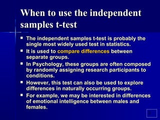
When to use the independent samplesWhen to use the independent samples
t-testt-test (cont.)(cont.)
Any differences between groups can beAny differences between groups can be
explored with the independent t-test, asexplored with the independent t-test, as
long as the tested members of each grouplong as the tested members of each group
are reasonably representative of theare reasonably representative of the
populationpopulation. [1]. [1]
[1][1] There are some technicalThere are some technical
requirements as well. Principally,requirements as well. Principally,
each variable must come from aeach variable must come from a
normal (or nearly normal) distribution.normal (or nearly normal) distribution.](https://image.slidesharecdn.com/04aindependentsamplet-test-140717045118-phpapp01/85/Independent-sample-t-test-3-320.jpg)


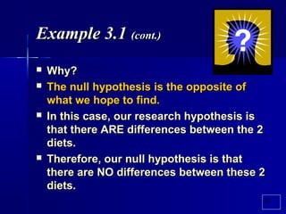


The document describes how to conduct an independent samples t-test. It explains that the t-test is used to compare differences between separate groups. An example is provided where participants are randomly assigned to either a pizza or beer diet for a week, and their weight gain is measured. Calculations are shown to find the variance, mean, and t-value for each group. The results indicate participants on the beer diet gained significantly more weight than those on the pizza diet, t(8) = 4.47, p < .05. Instructions are also provided for conducting this analysis in SPSS.