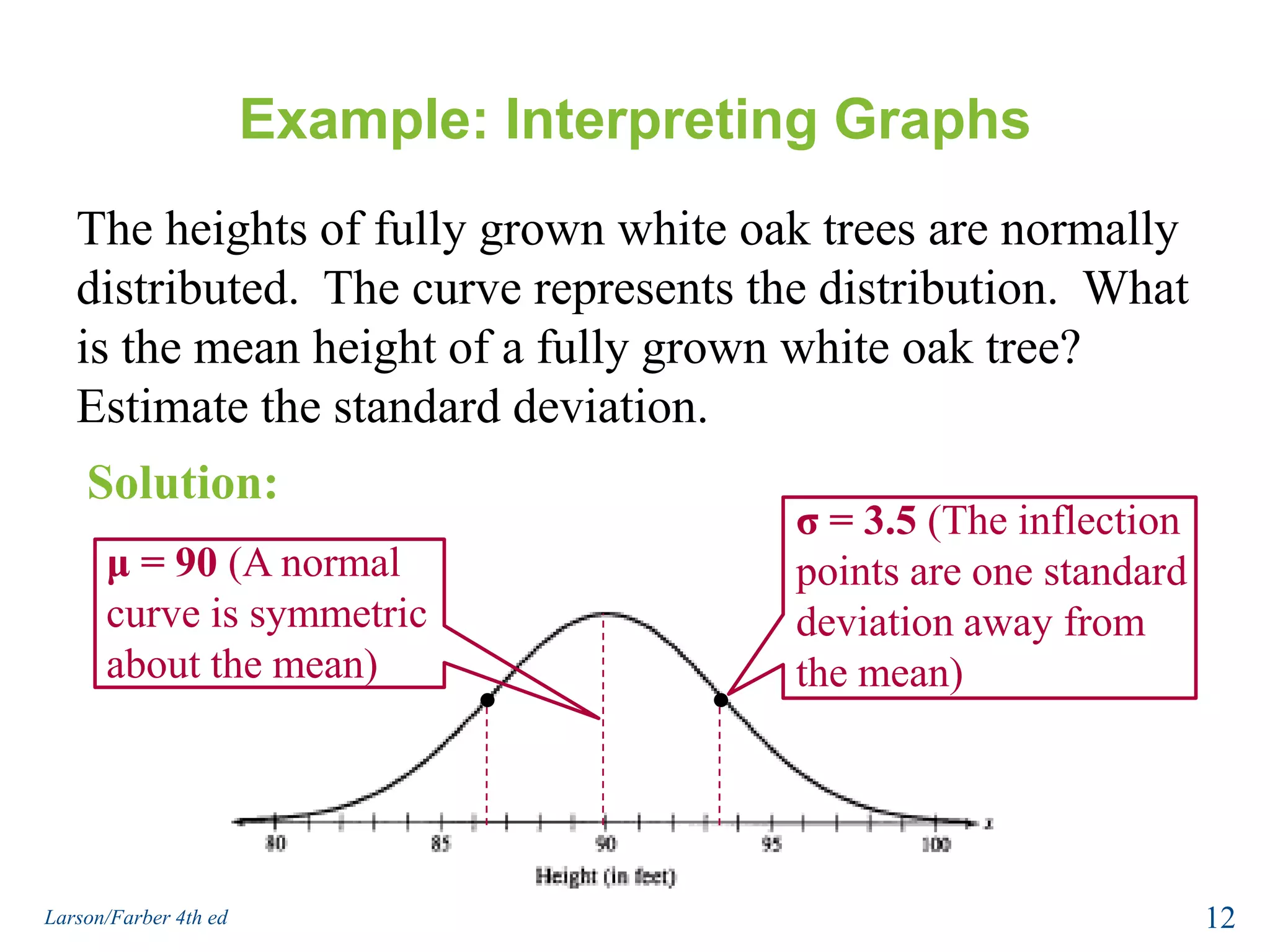
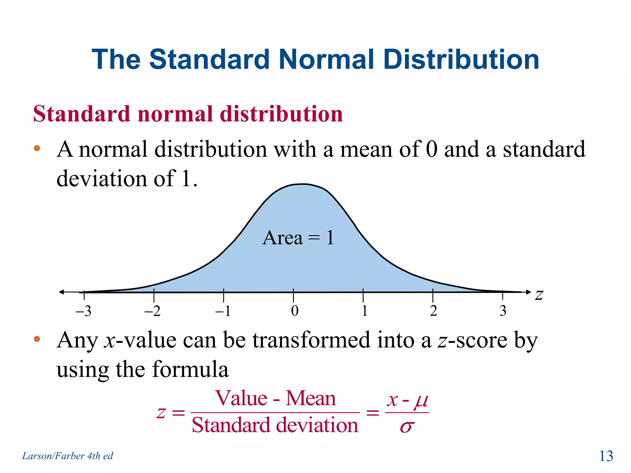
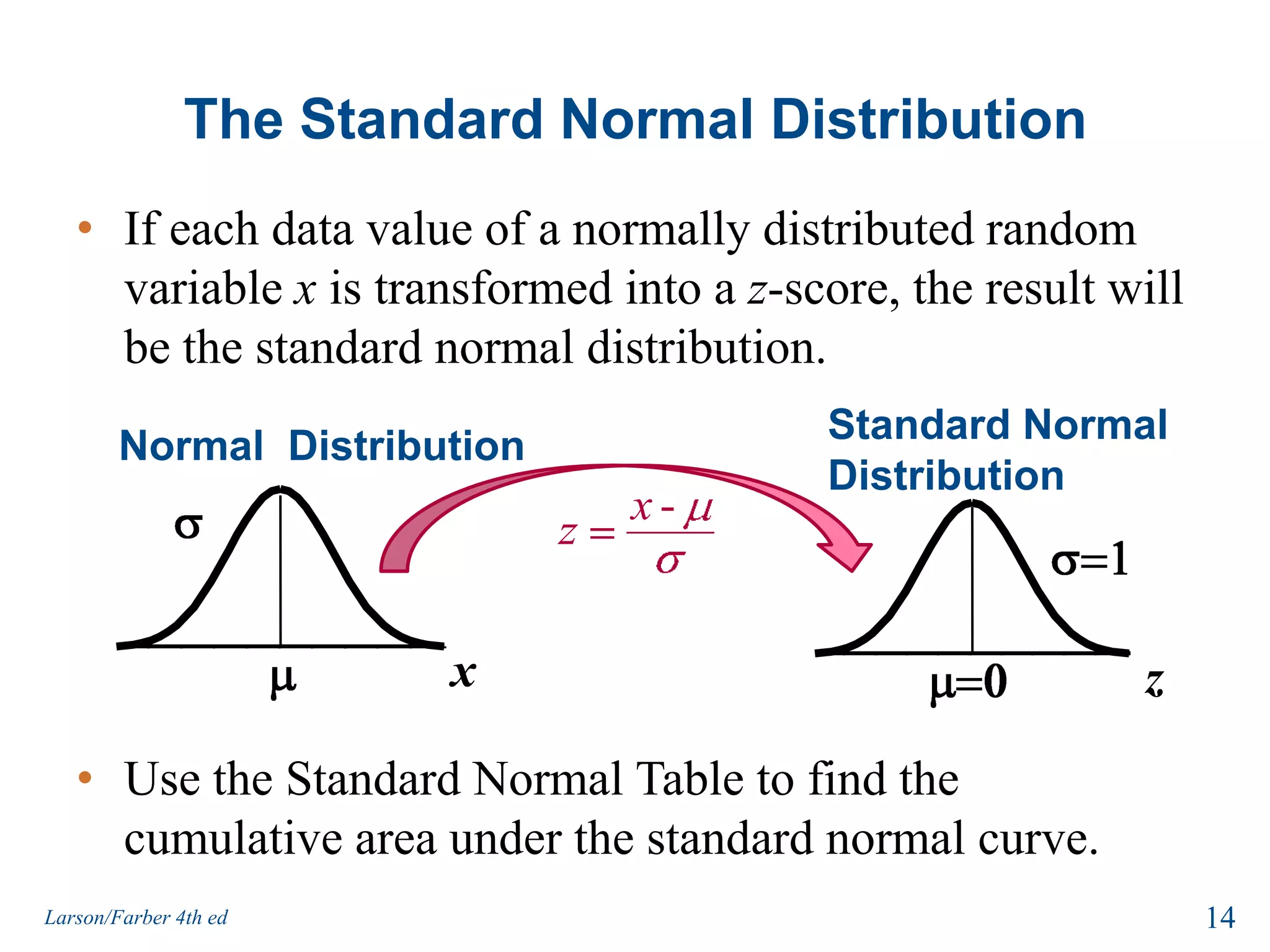
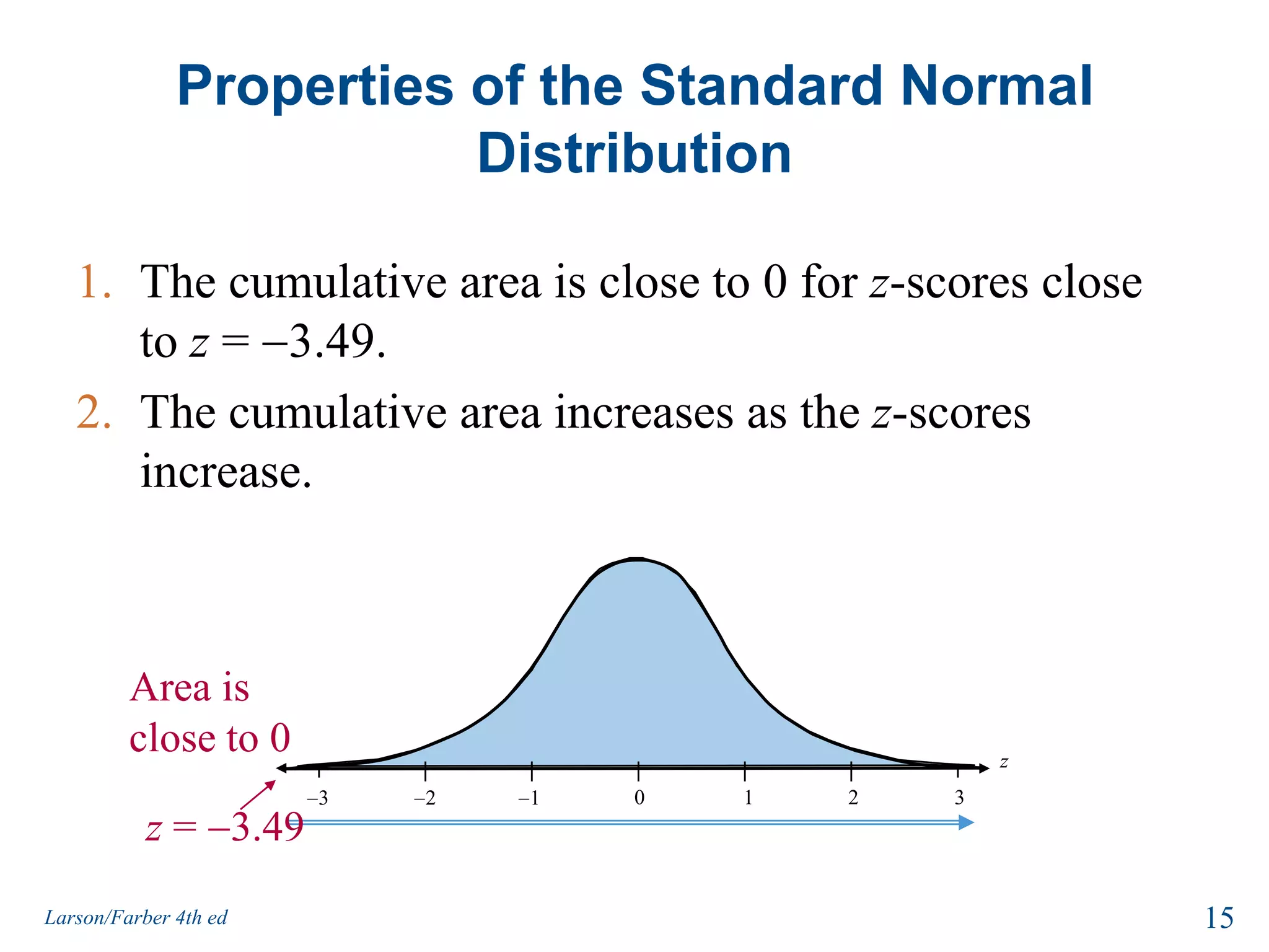
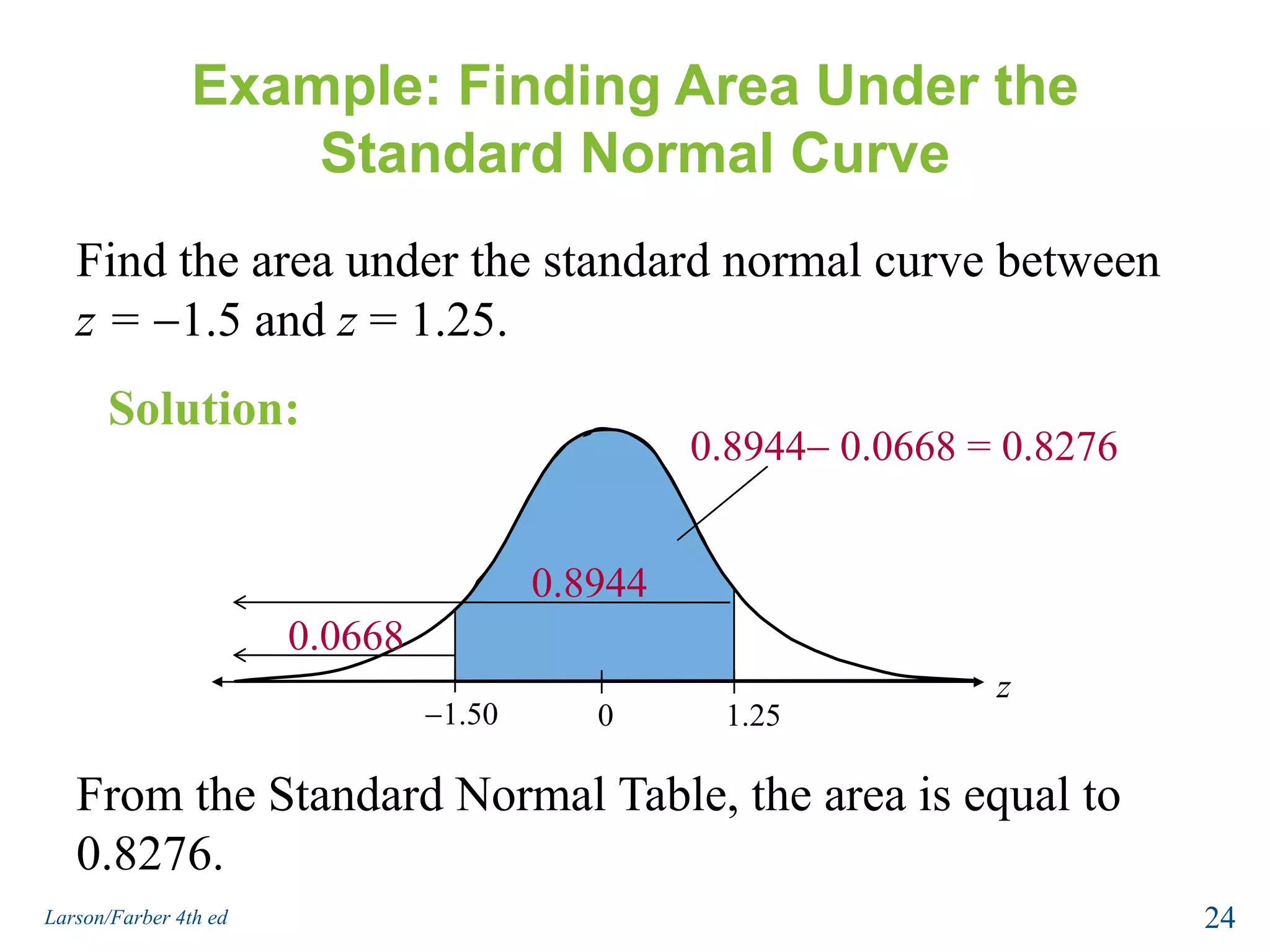
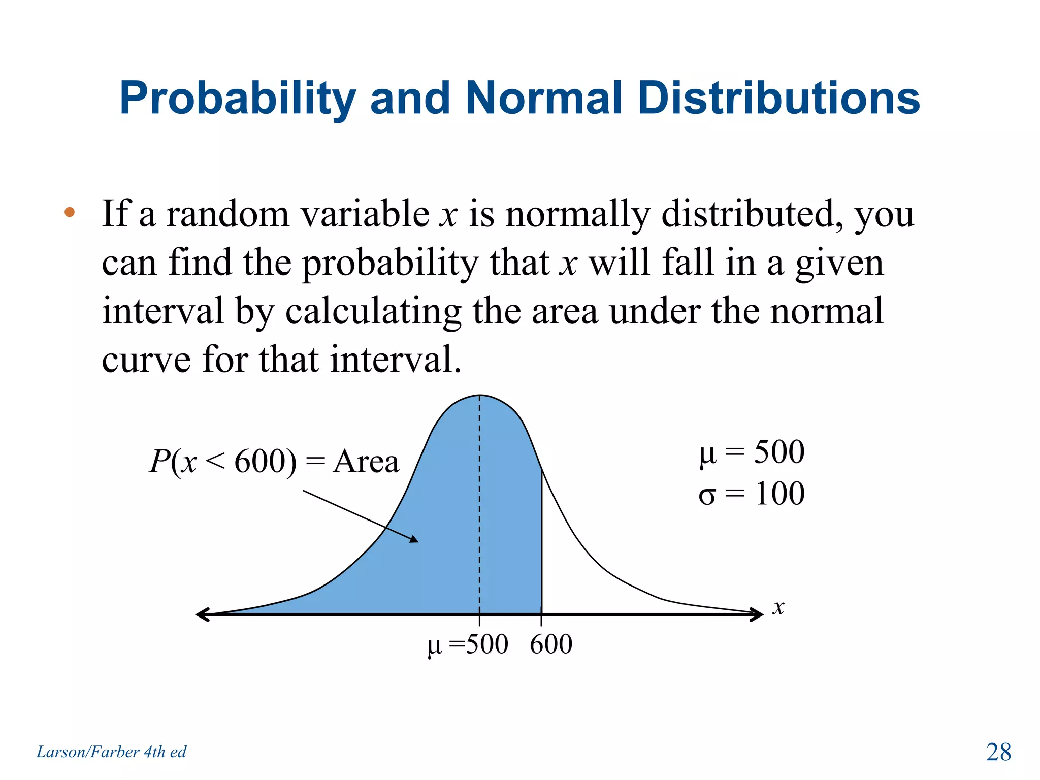
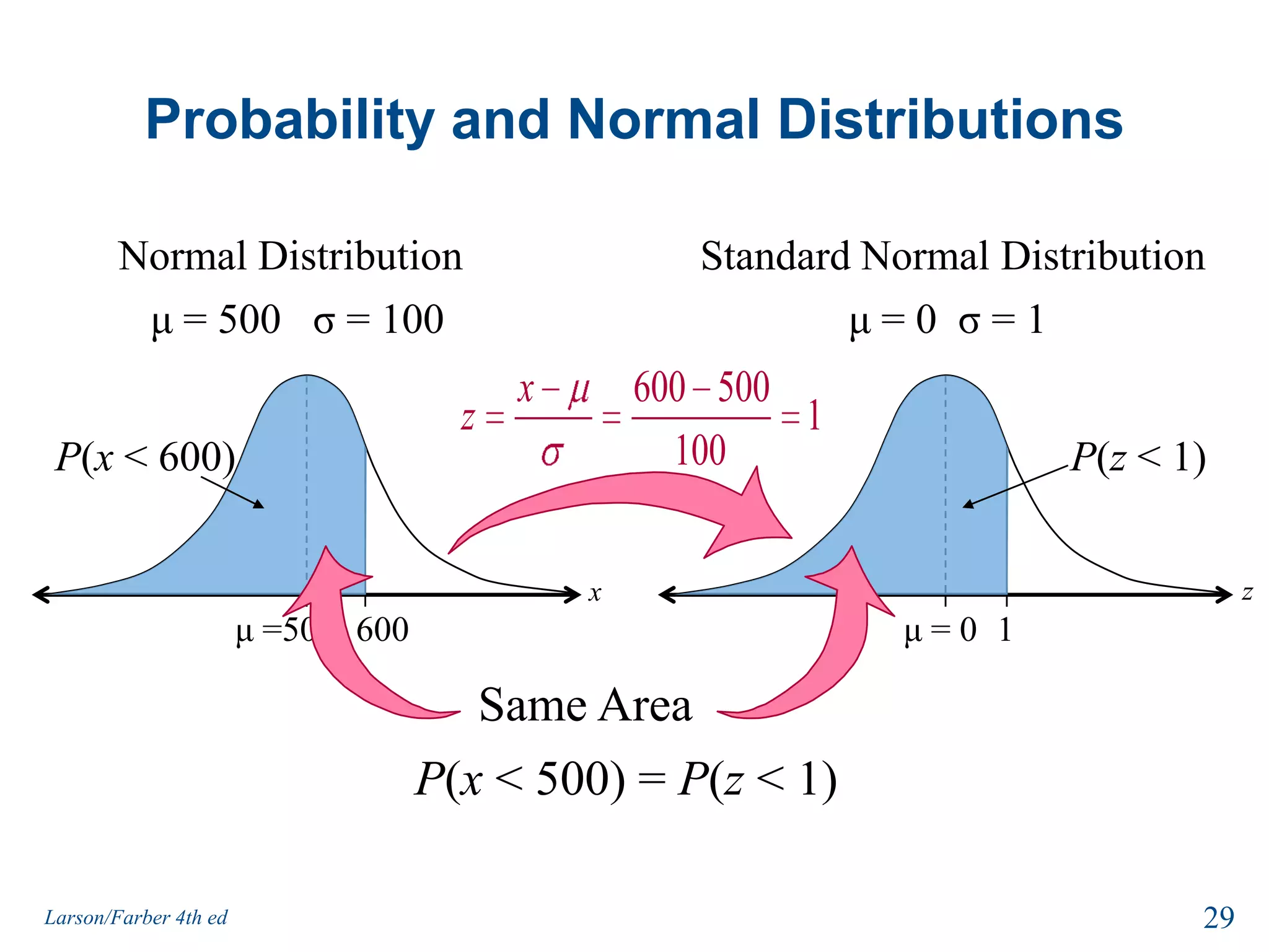
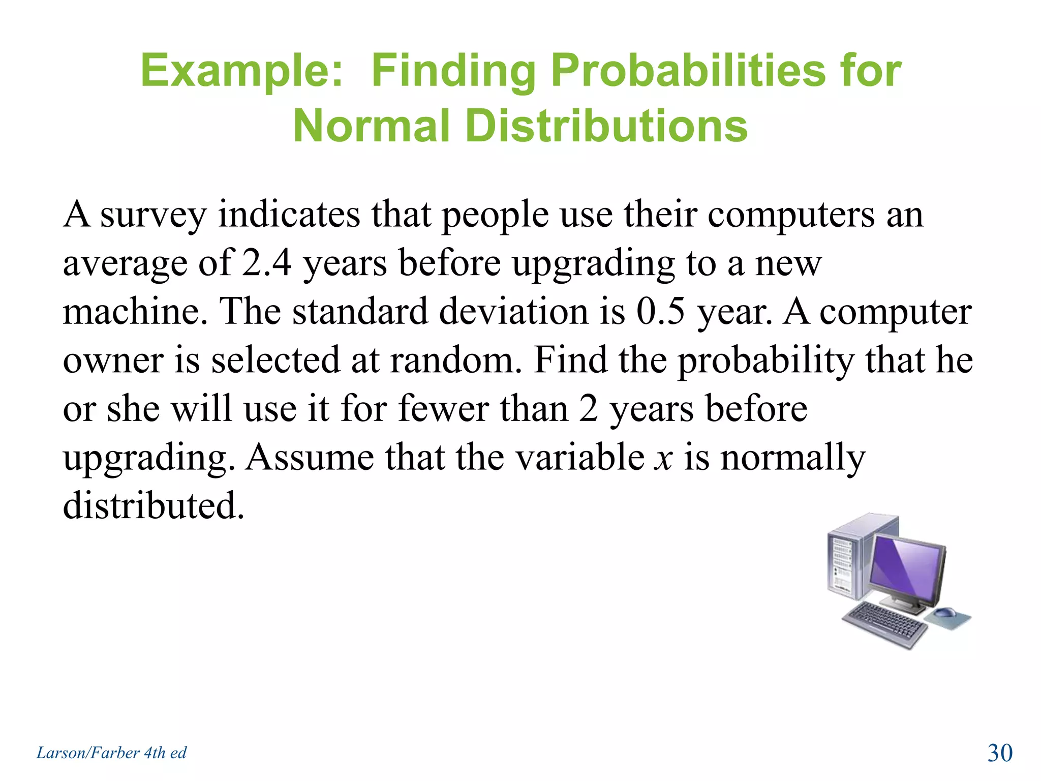
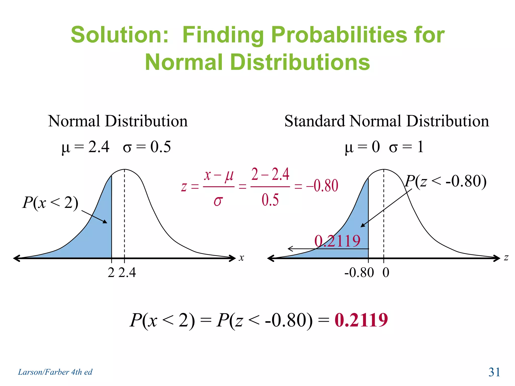
This document provides an overview of Chapter 5 from the textbook, which covers normal probability distributions. Section 5.1 introduces normal distributions and the standard normal distribution, including their key properties and how to interpret related graphs. It describes how any normal distribution can be transformed into a standard normal distribution for calculation purposes. Section 5.1 also shows how to find areas under the standard normal curve using the standard normal table. Section 5.2 discusses how to calculate probabilities for normally distributed variables by relating them to areas under the normal curve. It provides examples of finding probabilities and expected values.

1. Chapter 5Normal Probability Distributions1Larson/Farber 4th ed

2. Chapter Outline5.1 Introduction to Normal Distributions and the Standard Normal Distribution5.2 Normal Distributions: Finding Probabilities5.3 Normal Distributions: Finding Values5.4 Sampling Distributions and the Central Limit Theorem5.5 Normal Approximations to Binomial Distributions2Larson/Farber 4th ed

3. Section 5.1Introduction to Normal Distributions3Larson/Farber 4th ed

4. Section 5.1 ObjectivesInterpret graphs of normal probability distributionsFind areas under the standard normal curve4Larson/Farber 4th ed

5. Properties of a Normal DistributionContinuous random variableHas an infinite number of possible values that can be represented by an interval on the number line.Continuous probability distributionThe probability distribution of a continuous random variable.Hours spent studying in a day06391512182421The time spent studying can be any number between 0 and 24.5Larson/Farber 4th ed

6. Properties of Normal DistributionsNormal distribution A continuous probability distribution for a random variable, x. The most important continuous probability distribution in statistics.The graph of a normal distribution is called the normal curve.x6Larson/Farber 4th ed

7. Properties of Normal DistributionsThe mean, median, and mode are equal.The normal curve is bell-shaped and symmetric about the mean.The total area under the curve is equal to one.The normal curve approaches, but never touches the x-axis as it extends farther and farther away from the mean.Total area = 1xμ7Larson/Farber 4th ed

8. Properties of Normal DistributionsBetween μ – σ and μ + σ (in the center of the curve), the graph curves downward. The graph curves upward to the left of μ – σ and to the right of μ + σ. The points at which the curve changes from curving upward to curving downward are called the inflection points. Inflection pointsxμ+ σμμ+ 2σμ+ 3σμ 3σμ 2σμ σ8Larson/Farber 4th ed

9. Means and Standard DeviationsA normal distribution can have any mean and any positive standard deviation.The mean gives the location of the line of symmetry.The standard deviation describes the spread of the data.μ = 3.5σ = 1.5μ = 3.5σ = 0.7μ = 1.5σ = 0.79Larson/Farber 4th ed

10. Example: Understanding Mean and Standard DeviationWhich curve has the greater mean?Solution:Curve A has the greater mean (The line of symmetry of curve A occurs at x = 15. The line of symmetry of curve B occurs at x = 12.)10Larson/Farber 4th ed

11. Example: Understanding Mean and Standard DeviationWhich curve has the greater standard deviation?Solution:Curve B has the greater standard deviation (Curve B is more spread out than curve A.)11Larson/Farber 4th ed

12. Example: Interpreting GraphsThe heights of fully grown white oak trees are normally distributed. The curve represents the distribution. What is the mean height of a fully grown white oak tree? Estimate the standard deviation.Solution:σ = 3.5 (The inflection points are one standard deviation away from the mean) μ = 90 (A normal curve is symmetric about the mean)12Larson/Farber 4th ed

13. The Standard Normal Distributionz1023321Standard normal distributionA normal distribution with a mean of 0 and a standard deviation of 1.Area = 1Any x-value can be transformed into a z-score by using the formula 13Larson/Farber 4th ed

14. The Standard Normal DistributionsxmIf each data value of a normally distributed random variable x is transformed into a z-score, the result will be the standard normal distribution.Standard Normal DistributionNormal Distributions=1Use the Standard Normal Table to find the cumulative area under the standard normal curve.zm=014Larson/Farber 4th ed

15. Properties of the Standard Normal Distributionz1023321z = 3.49The cumulative area is close to 0 for z-scores close to z = 3.49.The cumulative area increases as the z-scores increase.Area is close to 015Larson/Farber 4th ed

16. Properties of the Standard Normal DistributionArea is close to 1z1023321z = 3.49z = 0Area is 0.5000The cumulative area for z = 0 is 0.5000.The cumulative area is close to 1 for z-scores close to z = 3.49.16Larson/Farber 4th ed

17. Example: Using The Standard Normal TableFind the cumulative area that corresponds to a z-score of 1.15.Solution:Find 1.1 in the left hand column.Move across the row to the column under 0.05The area to the left of z = 1.15 is 0.8749.17Larson/Farber 4th ed

18. Example: Using The Standard Normal TableFind the cumulative area that corresponds to a z-score of -0.24.Solution:Find -0.2 in the left hand column.Move across the row to the column under 0.04The area to the left of z = -0.24 is 0.4052.18Larson/Farber 4th ed

19. Finding Areas Under the Standard Normal CurveSketch the standard normal curve and shade the appropriate area under the curve.Find the area by following the directions for each case shown.To find the area to the left of z, find the area that corresponds to z in the Standard Normal Table.The area to the left of z = 1.23 is 0.8907Use the table to find the area for the z-score19Larson/Farber 4th ed

20. Finding Areas Under the Standard Normal CurveSubtract to find the area to the right of z = 1.23: 1  0.8907 = 0.1093.Use the table to find the area for the z-score.To find the area to the right of z, use the Standard Normal Table to find the area that corresponds to z. Then subtract the area from 1.The area to the left of z = 1.23 is 0.8907.20Larson/Farber 4th ed

21. Finding Areas Under the Standard Normal CurveSubtract to find the area of the region between the two z-scores: 0.8907  0.2266 = 0.6641.The area to the left of z = 1.23 is 0.8907.The area to the left of z = 0.75 is 0.2266.Use the table to find the area for the z-scores.To find the area between two z-scores, find the area corresponding to each z-score in the Standard Normal Table. Then subtract the smaller area from the larger area.21Larson/Farber 4th ed

22. Example: Finding Area Under the Standard Normal CurveFind the area under the standard normal curve to the left of z = -0.99.Solution:0.1611z0.99 0From the Standard Normal Table, the area is equal to 0.1611.22Larson/Farber 4th ed

23. Example: Finding Area Under the Standard Normal Curve1  0.8554 = 0.1446z1.060Find the area under the standard normal curve to the right of z = 1.06.Solution:0.8554From the Standard Normal Table, the area is equal to 0.1446.23Larson/Farber 4th ed

24. Example: Finding Area Under the Standard Normal Curve0.8944 0.0668 = 0.8276z1.501.250Find the area under the standard normal curve between z = 1.5 and z = 1.25.Solution:0.06680.8944From the Standard Normal Table, the area is equal to 0.8276.24Larson/Farber 4th ed

25. Section 5.1 SummaryInterpreted graphs of normal probability distributionsFound areas under the standard normal curve25Larson/Farber 4th ed

26. Section 5.2Normal Distributions: Finding Probabilities26Larson/Farber 4th ed

27. Section 5.2 ObjectivesFind probabilities for normally distributed variables27Larson/Farber 4th ed

28. Probability and Normal Distributionsμ = 500σ = 100P(x < 600) = Areax600μ =500If a random variable x is normally distributed, you can find the probability that x will fall in a given interval by calculating the area under the normal curve for that interval.28Larson/Farber 4th ed

29. Probability and Normal DistributionsNormal DistributionStandard Normal Distributionμ = 500 σ = 100μ = 0 σ = 1P(x < 600)P(z < 1)zxSame Area600μ =5001μ = 0P(x < 500) = P(z < 1)29Larson/Farber 4th ed

30. Example: Finding Probabilities for Normal DistributionsA survey indicates that people use their computers an average of 2.4 years before upgrading to a new machine. The standard deviation is 0.5 year. A computer owner is selected at random. Find the probability that he or she will use it for fewer than 2 years before upgrading. Assume that the variable x is normally distributed.30Larson/Farber 4th ed

31. Solution: Finding Probabilities for Normal DistributionsNormal DistributionStandard Normal Distributionμ = 2.4 σ = 0.5μ = 0 σ = 1P(z < -0.80)P(x < 2)0.2119zx22.4-0.800P(x < 2) = P(z < -0.80) = 0.211931Larson/Farber 4th ed

32. Example: Finding Probabilities for Normal DistributionsA survey indicates that for each trip to the supermarket, a shopper spends an average of 45 minutes with a standard deviation of 12 minutes in the store. The length of time spent in the store is normally distributed and is represented by the variable x. A shopper enters the store. Find the probability that the shopper will be in the store for between 24 and 54 minutes.32Larson/Farber 4th ed

33. Solution: Finding Probabilities for Normal DistributionsP(-1.75 < z < 0.75)P(24 < x < 54)xz2445-1.750Normal Distributionμ = 45 σ = 12Standard Normal Distributionμ = 0 σ = 10.04010.77340.7554P(24 < x < 54) = P(-1.75 < z < 0.75) = 0.7734 – 0.0401 = 0.733333Larson/Farber 4th ed

34. Example: Finding Probabilities for Normal DistributionsFind the probability that the shopper will be in the store more than 39 minutes. (Recall μ = 45 minutes and σ = 12 minutes)34Larson/Farber 4th ed

35. Solution: Finding Probabilities for Normal DistributionsP(z > -0.50)P(x > 39)xz39450Normal Distributionμ = 45 σ = 12Standard Normal Distributionμ = 0 σ = 10.3085-0.50P(x > 39) = P(z > -0.50) = 1– 0.3085 = 0.691535Larson/Farber 4th ed

36. Example: Finding Probabilities for Normal DistributionsIf 200 shoppers enter the store, how many shoppers would you expect to be in the store more than 39 minutes?Solution:Recall P(x > 39) = 0.6915200(0.6915) =138.3 (or about 138) shoppers36Larson/Farber 4th ed

37. Example: Using Technology to find Normal ProbabilitiesAssume that cholesterol levels of men in the United States are normally distributed, with a mean of 215 milligrams per deciliter and a standard deviation of 25 milligrams per deciliter. You randomly select a man from the United States. What is the probability that his cholesterol level is less than 175? Use a technology tool to find the probability.37Larson/Farber 4th ed

38. Solution: Using Technology to find Normal ProbabilitiesMust specify the mean, standard deviation, and the x-value(s) that determine the interval.38Larson/Farber 4th ed

39. Section 5.2 SummaryFound probabilities for normally distributed variables39Larson/Farber 4th ed

40. Section 5.3Normal Distributions: Finding Values40Larson/Farber 4th ed

41. Section 5.3 ObjectivesFind a z-score given the area under the normal curveTransform a z-score to an x-valueFind a specific data value of a normal distribution given the probability41Larson/Farber 4th ed

42. Finding values Given a ProbabilityIn section 5.2 we were given a normally distributed random variable x and we were asked to find a probability.In this section, we will be given a probability and we will be asked to find the value of the random variable x.5.2probabilityxz5.342Larson/Farber 4th ed

43. Example: Finding a z-Score Given an AreaFind the z-score that corresponds to a cumulative area of 0.3632.Solution:0.3632zz043Larson/Farber 4th ed

44. Solution: Finding a z-Score Given an AreaLocate 0.3632 in the body of the Standard Normal Table. The z-score is -0.35.The values at the beginning of the corresponding row and at the top of the column give the z-score.44Larson/Farber 4th ed

45. Example: Finding a z-Score Given an AreaFind the z-score that has 10.75% of the distribution’s area to its right.Solution:1 – 0.1075 = 0.89250.1075zz0Because the area to the right is 0.1075, the cumulative area is 0.8925.45Larson/Farber 4th ed

46. Solution: Finding a z-Score Given an AreaLocate 0.8925 in the body of the Standard Normal Table. The z-score is 1.24.The values at the beginning of the corresponding row and at the top of the column give the z-score.46Larson/Farber 4th ed

47. Example: Finding a z-Score Given a Percentile0.05zz 0Find the z-score that corresponds to P5.Solution:The z-score that corresponds to P5 is the same z-score that corresponds to an area of 0.05.The areas closest to 0.05 in the table are 0.0495 (z = -1.65) and 0.0505 (z = -1.64). Because 0.05 is halfway between the two areas in the table, use the z-score that is halfway between -1.64 and -1.65. The z-score is -1.645.47Larson/Farber 4th ed

48. Transforming a z-Score to an x-ScoreTo transform a standard z-score to a data value x in a given population, use the formulax = μ + zσ48Larson/Farber 4th ed

49. Example: Finding an x-ValueThe speeds of vehicles along a stretch of highway are normally distributed, with a mean of 67 miles per hour and a standard deviation of 4 miles per hour. Find the speeds x corresponding to z-sores of 1.96, -2.33, and 0.Solution: Use the formula x = μ + zσz = 1.96: x = 67 + 1.96(4) = 74.84 miles per hour

50. z = -2.33: x = 67 + (-2.33)(4) = 57.68 miles per hour

51. z = 0: x = 67 + 0(4) = 67 miles per hourNotice 74.84 mph is above the mean, 57.68 mph is below the mean, and 67 mph is equal to the mean.49Larson/Farber 4th ed

52. Example: Finding a Specific Data Value5%x?75Scores for a civil service exam are normally distributed, with a mean of 75 and a standard deviation of 6.5. To be eligible for civil service employment, you must score in the top 5%. What is the lowest score you can earn and still be eligible for employment?Solution:An exam score in the top 5% is any score above the 95th percentile. Find the z-score that corresponds to a cumulative area of 0.95.1 – 0.05 = 0.95z? 050Larson/Farber 4th ed

53. Solution: Finding a Specific Data Value5%x?75From the Standard Normal Table, the areas closest to 0.95 are 0.9495 (z = 1.64) and 0.9505 (z = 1.65). Because 0.95 is halfway between the two areas in the table, use the z-score that is halfway between 1.64 and 1.65. That is, z = 1.645.z1.645 051Larson/Farber 4th ed

54. Solution: Finding a Specific Data Value5%x85.6975Using the equation x = μ + zσx = 75 + 1.645(6.5) ≈ 85.69z1.645 0The lowest score you can earn and still be eligible for employment is 86.52Larson/Farber 4th ed

55. Section 5.3 SummaryFound a z-score given the area under the normal curveTransformed a z-score to an x-valueFound a specific data value of a normal distribution given the probability53Larson/Farber 4th ed

56. Section 5.4Sampling Distributions and the Central Limit Theorem54Larson/Farber 4th ed

57. Section 5.4 ObjectivesFind sampling distributions and verify their propertiesInterpret the Central Limit TheoremApply the Central Limit Theorem to find the probability of a sample mean55Larson/Farber 4th ed

58. Sampling DistributionsSampling distributionThe probability distribution of a sample statistic. Formed when samples of size n are repeatedly taken from a population. e.g. Sampling distribution of sample means56Larson/Farber 4th ed

59. Sampling Distribution of Sample MeansPopulation with μ, σSample 3The sampling distribution consists of the values of the sample means, Sample 1Sample 2Sample 4 Sample 557Larson/Farber 4th ed

60. The mean of the sample means, , is equal to the population mean μ. The standard deviation of the sample means, , is equal to the population standard deviation, σ divided by the square root of the sample size, n. Properties of Sampling Distributions of Sample MeansCalled the standard error of the mean.58Larson/Farber 4th ed

61. Example: Sampling Distribution of Sample MeansThe population values {1, 3, 5, 7} are written on slips of paper and put in a box. Two slips of paper are randomly selected, with replacement. Find the mean, variance, and standard deviation of the population.Solution:59Larson/Farber 4th ed

62. Example: Sampling Distribution of Sample MeansProbability Histogram of Population of xP(x)0.25Probabilityx1357Population valuesGraph the probability histogram for the population values.Solution:All values have the same probability of being selected (uniform distribution)60Larson/Farber 4th ed

63. Example: Sampling Distribution of Sample MeansList all the possible samples of size n = 2 and calculate the mean of each sample.Solution:SampleSample11, 135, 1These means form the sampling distribution of sample means.21, 345, 331, 555, 541, 765, 723, 147, 133, 357, 343, 567, 553, 777, 761Larson/Farber 4th ed

64. Example: Sampling Distribution of Sample MeansConstruct the probability distribution of the sample means.Solution:fProbability62Larson/Farber 4th ed

65. Example: Sampling Distribution of Sample MeansFind the mean, variance, and standard deviation of the sampling distribution of the sample means.Solution:The mean, variance, and standard deviation of the 16 sample means are:These results satisfy the properties of sampling distributions of sample means.63Larson/Farber 4th ed

66. Example: Sampling Distribution of Sample MeansProbability Histogram of Sampling Distribution ofP(x)0.250.20Probability0.150.100.05432567Sample meanGraph the probability histogram for the sampling distribution of the sample means.Solution:The shape of the graph is symmetric and bell shaped. It approximates a normal distribution.64Larson/Farber 4th ed

67. The Central Limit TheoremxxIf samples of size n 30, are drawn from any population with mean =  and standard deviation = ,then the sampling distribution of the sample means approximates a normal distribution. The greater the sample size, the better the approximation.65Larson/Farber 4th ed

68. The Central Limit TheoremxxIf the population itself is normally distributed, the sampling distribution of the sample means is normally distribution for any sample size n.66Larson/Farber 4th ed

69. The Central Limit TheoremIn either case, the sampling distribution of sample means has a mean equal to the population mean.The sampling distribution of sample means has a variance equal to 1/n times the variance of the population and a standard deviation equal to the population standard deviation divided by the square root of n.VarianceStandard deviation (standard error of the mean)67Larson/Farber 4th ed

70. The Central Limit TheoremAny Population DistributionNormal Population DistributionDistribution of Sample Means, n ≥ 30Distribution of Sample Means, (any n) 68Larson/Farber 4th ed

71. Example: Interpreting the Central Limit TheoremPhone bills for residents of a city have a mean of $64 and a standard deviation of $9. Random samples of 36 phone bills are drawn from this population and the mean of each sample is determined. Find the mean and standard error of the mean of the sampling distribution. Then sketch a graph of the sampling distribution of sample means.69Larson/Farber 4th ed

72. Solution: Interpreting the Central Limit TheoremThe mean of the sampling distribution is equal to the population meanThe standard error of the mean is equal to the population standard deviation divided by the square root of n.70Larson/Farber 4th ed

73. Solution: Interpreting the Central Limit TheoremSince the sample size is greater than 30, the sampling distribution can be approximated by a normal distribution with 71Larson/Farber 4th ed

74. Example: Interpreting the Central Limit TheoremThe heights of fully grown white oak trees are normally distributed, with a mean of 90 feet and standard deviation of 3.5 feet. Random samples of size 4 are drawn from this population, and the mean of each sample is determined. Find the mean and standard error of the mean of the sampling distribution. Then sketch a graph of the sampling distribution of sample means.72Larson/Farber 4th ed

75. Solution: Interpreting the Central Limit TheoremThe mean of the sampling distribution is equal to the population meanThe standard error of the mean is equal to the population standard deviation divided by the square root of n.73Larson/Farber 4th ed

76. Solution: Interpreting the Central Limit TheoremSince the population is normally distributed, the sampling distribution of the sample means is also normally distributed.74Larson/Farber 4th ed

77. Probability and the Central Limit TheoremTo transform x to a z-score75Larson/Farber 4th ed

78. Example: Probabilities for Sampling DistributionsThe graph shows the length of time people spend driving each day. You randomly select 50 drivers age 15 to 19. What is the probability that the mean time they spend driving each day is between 24.7 and 25.5 minutes? Assume that σ = 1.5 minutes.76Larson/Farber 4th ed

79. Solution: Probabilities for Sampling DistributionsFrom the Central Limit Theorem (sample size is greater than 30), the sampling distribution of sample means is approximately normal with 77Larson/Farber 4th ed

80. Solution: Probabilities for Sampling DistributionsP(-1.41 < z < 2.36)P(24.7 < x < 25.5)xz24.725-1.410Normal Distributionμ = 25 σ = 0.21213Standard Normal Distributionμ = 0 σ = 10.99090.07932.3625.578Larson/Farber 4th edP(24 < x < 54) = P(-1.41 < z < 2.36) = 0.9909 – 0.0793 = 0.9116

81. Example: Probabilities for x and xA bank auditor claims that credit card balances are normally distributed, with a mean of $2870 and a standard deviation of $900.What is the probability that a randomly selected credit card holder has a credit card balance less than $2500?Solution:You are asked to find the probability associated with a certain value of the random variable x.79Larson/Farber 4th ed

82. Solution: Probabilities for x and xP(x < 2500)P(z < -0.41)xz25002870-0.410Normal Distributionμ = 2870 σ = 900Standard Normal Distributionμ = 0 σ = 10.3409P( x < 2500) = P(z < -0.41) = 0.340980Larson/Farber 4th ed

83. Example: Probabilities for x and xYou randomly select 25 credit card holders. What is the probability that their mean credit card balance is less than $2500?Solution:You are asked to find the probability associated with a sample mean .81Larson/Farber 4th ed

84. P(x < 2500)zx-2.06Solution: Probabilities for x and x25002870Standard Normal Distributionμ = 0 σ = 1Normal Distributionμ = 2870 σ = 180P(z < -2.06)0.01970P( x < 2500) = P(z < -2.06) = 0.019782Larson/Farber 4th ed

85. Solution: Probabilities for x and xThere is a 34% chance that an individual will have a balance less than $2500.There is only a 2% chance that the mean of a sample of 25 will have a balance less than $2500 (unusual event). It is possible that the sample is unusual or it is possible that the auditor’s claim that the mean is $2870 is incorrect.83Larson/Farber 4th ed

86. Section 5.4 SummaryFound sampling distributions and verify their propertiesInterpreted the Central Limit TheoremApplied the Central Limit Theorem to find the probability of a sample mean84Larson/Farber 4th ed

87. Section 5.5Normal Approximations to Binomial Distributions85Larson/Farber 4th ed

88. Section 5.5 ObjectivesDetermine when the normal distribution can approximate the binomial distributionFind the correction for continuityUse the normal distribution to approximate binomial probabilities86Larson/Farber 4th ed

89. Normal Approximation to a BinomialThe normal distribution is used to approximate the binomial distribution when it would be impractical to use the binomial distribution to find a probability. Normal Approximation to a Binomial DistributionIf np 5 and nq  5, then the binomial random variable x is approximately normally distributed with mean μ = npstandard deviation87Larson/Farber 4th ed

90. Normal Approximation to a BinomialBinomial distribution: p = 0.25As n increases the histogram approaches a normal curve.88Larson/Farber 4th ed

91. Example: Approximating the BinomialDecide whether you can use the normal distribution to approximate x, the number of people who reply yes. If you can, find the mean and standard deviation.Fifty-one percent of adults in the U.S. whose New Year’s resolution was to exercise more achieved their resolution. You randomly select 65 adults in the U.S. whose resolution was to exercise more and ask each if he or she achieved that resolution.89Larson/Farber 4th ed

92. Solution: Approximating the BinomialYou can use the normal approximationn = 65, p = 0.51, q = 0.49np = (65)(0.51) = 33.15 ≥ 5nq = (65)(0.49) = 31.85 ≥ 5Mean: μ = np = 33.15Standard Deviation: 90Larson/Farber 4th ed

93. Example: Approximating the BinomialDecide whether you can use the normal distribution to approximate x, the number of people who reply yes. If you can find, find the mean and standard deviation.Fifteen percent of adults in the U.S. do not make New Year’s resolutions. You randomly select 15 adults in the U.S. and ask each if he or she made a New Year’s resolution.91Larson/Farber 4th ed

94. Solution: Approximating the BinomialYou cannot use the normal approximationn = 15, p = 0.15, q = 0.85np = (15)(0.15) = 2.25 < 5nq = (15)(0.85) = 12.75 ≥ 5Because np < 5, you cannot use the normal distribution to approximate the distribution of x.92Larson/Farber 4th ed

95. Correction for ContinuityThe binomial distribution is discrete and can be represented by a probability histogram. To calculate exact binomial probabilities, the binomial formula is used for each value of x and the results are added.Geometrically this corresponds to adding the areas of bars in the probability histogram.93Larson/Farber 4th ed

96. Correction for ContinuityWhen you use a continuous normal distribution to approximate a binomial probability, you need to move 0.5 unit to the left and right of the midpoint to include all possible x-values in the interval (correction for continuity).Exact binomial probabilityNormal approximationP(x = c)P(c – 0.5 < x < c + 0.5)ccc+ 0.5c– 0.594Larson/Farber 4th ed

97. Example: Using a Correction for ContinuityUse a correction for continuity to convert the binomial intervals to a normal distribution interval.The probability of getting between 270 and 310 successes, inclusive.Solution:The discrete midpoint values are 270, 271, …, 310.

98. The corresponding interval for the continuous normal distribution is269.5 < x < 310.595Larson/Farber 4th ed

99. Example: Using a Correction for ContinuityUse a correction for continuity to convert the binomial intervals to a normal distribution interval.The probability of getting at least 158 successes.Solution:The discrete midpoint values are 158, 159, 160, ….

100. The corresponding interval for the continuous normal distribution isx > 157.596Larson/Farber 4th ed

101. Example: Using a Correction for ContinuityUse a correction for continuity to convert the binomial intervals to a normal distribution interval.The probability of getting less than 63 successes.Solution:The discrete midpoint values are …,60, 61, 62.

102. The corresponding interval for the continuous normal distribution isx < 62.597Larson/Farber 4th ed

103. Using the Normal Distribution to Approximate Binomial Probabilities In Words In SymbolsVerify that the binomial distribution applies.Determine if you can use the normal distribution to approximate x, the binomial variable.Find the mean  and standard deviation for the distribution.Specify n, p, and q.Is np 5?Is nq 5?98Larson/Farber 4th ed

104. Using the Normal Distribution to Approximate Binomial Probabilities In Words In SymbolsApply the appropriate continuity correction. Shade the corresponding area under the normal curve.Find the corresponding z-score(s).Find the probability. Add or subtract 0.5 from endpoints. Use the Standard Normal Table.99Larson/Farber 4th ed

105. Example: Approximating a Binomial ProbabilityFifty-one percent of adults in the U. S. whose New Year’s resolution was to exercise more achieved their resolution. You randomly select 65 adults in the U. S. whose resolution was to exercise more and ask each if he or she achieved that resolution. What is the probability that fewer than forty of them respond yes? (Source: Opinion Research Corporation)Solution:Can use the normal approximation (see slide 89)μ = 65∙0.51 = 33.15 100Larson/Farber 4th ed

106. Solution: Approximating a Binomial ProbabilityApply the continuity correction: Fewer than 40 (…37, 38, 39) corresponds to the continuous normal distribution interval x < 39.5Normal Distributionμ = 33.15 σ = 4.03Standard Normalμ = 0 σ = 1P(z < 1.58)P(x < 39.5)xz39.5μ =33.151.58μ =00.9429P(z < 1.58) = 0.9429101Larson/Farber 4th ed

107. Example: Approximating a Binomial ProbabilityA survey reports that 86% of Internet users use Windows® Internet Explorer ® as their browser. You randomly select 200 Internet users and ask each whether he or she uses Internet Explorer as his or her browser. What is the probability that exactly 176 will say yes? (Source: 0neStat.com)Solution:Can use the normal approximationnp = (200)(0.86) = 172 ≥ 5 nq = (200)(0.14) = 28 ≥ 5 μ = 200∙0.86 = 172 102Larson/Farber 4th ed

108. Apply the continuity correction: Exactly 176 corresponds to the continuous normal distribution interval 175.5 < x < 176.5Solution: Approximating a Binomial ProbabilityNormal Distributionμ = 172 σ = 4.91Standard Normalμ = 0 σ = 1P(175.5 < x < 176.5)P(0.71 < z < 0.92)x176.5μ =172z0.76110.82120.92μ =00.71175.5P(0.71 < z < 0.92) = 0.8212 – 0.7611 = 0.0601103Larson/Farber 4th ed

109. Section 5.5 SummaryDetermined when the normal distribution can approximate the binomial distributionFound the correction for continuityUsed the normal distribution to approximate binomial probabilities104Larson/Farber 4th ed