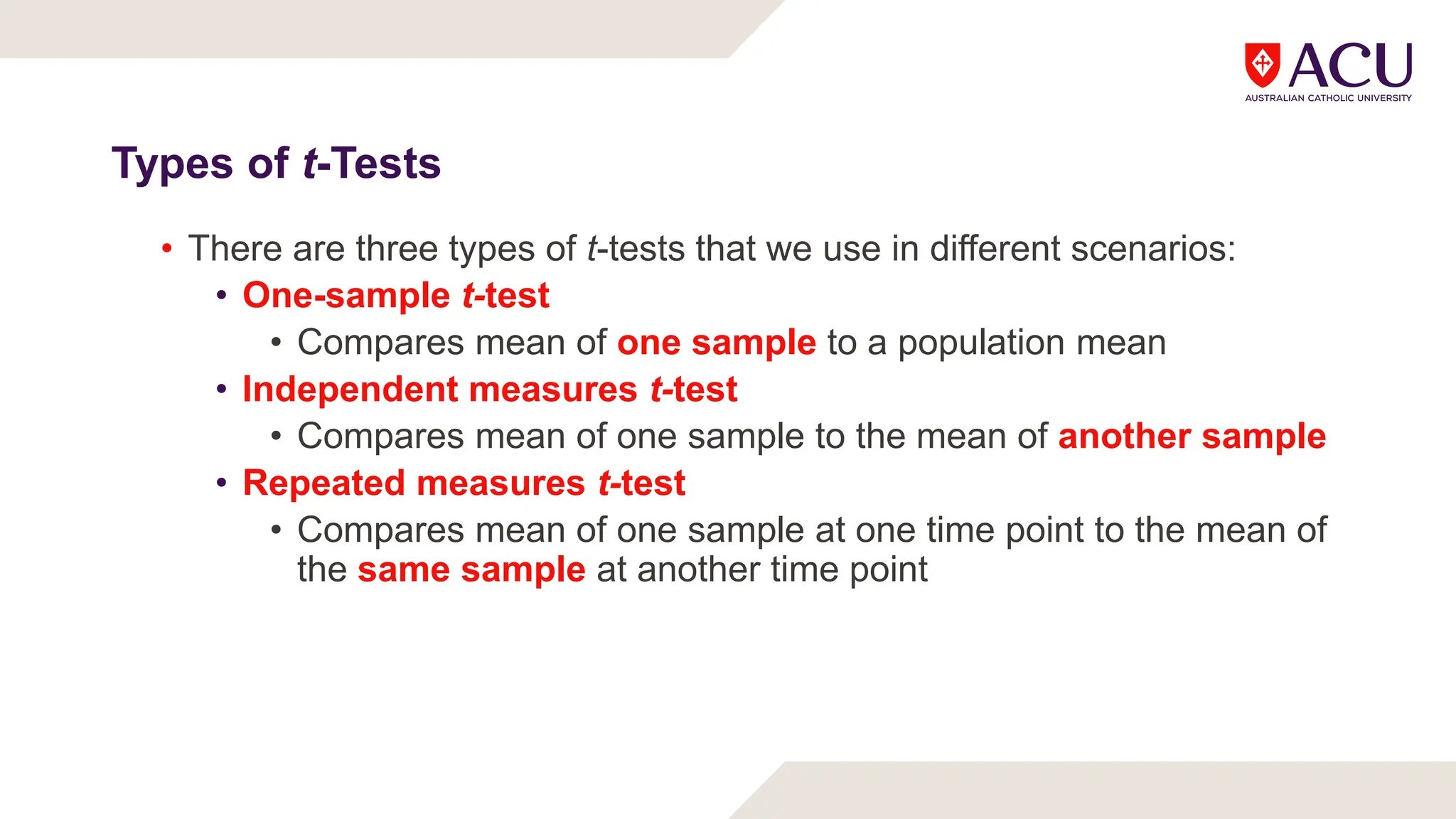
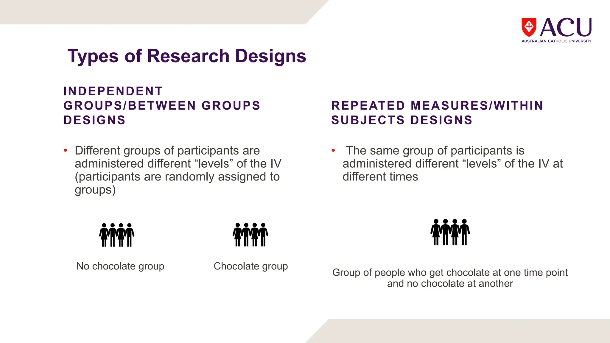
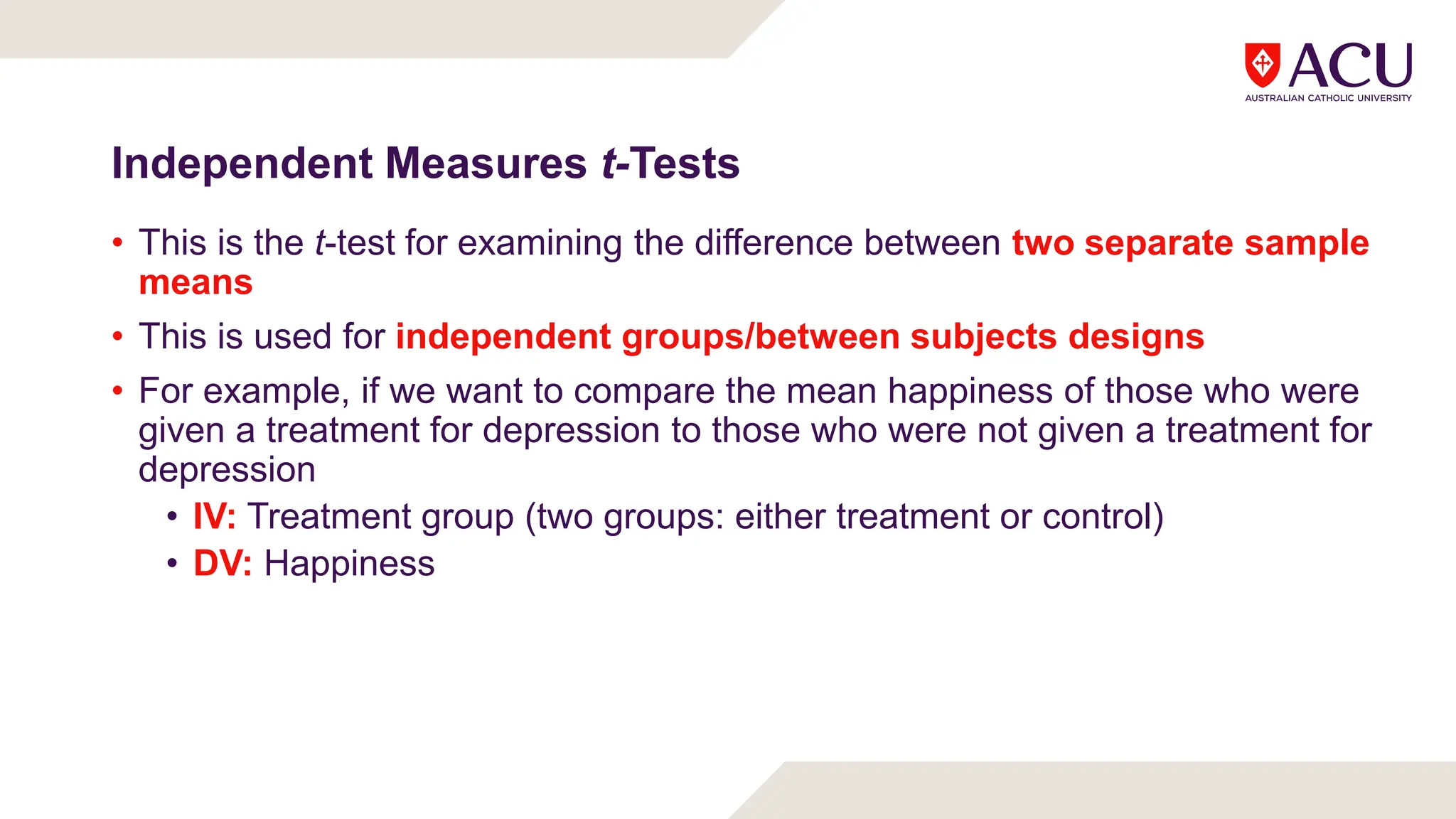
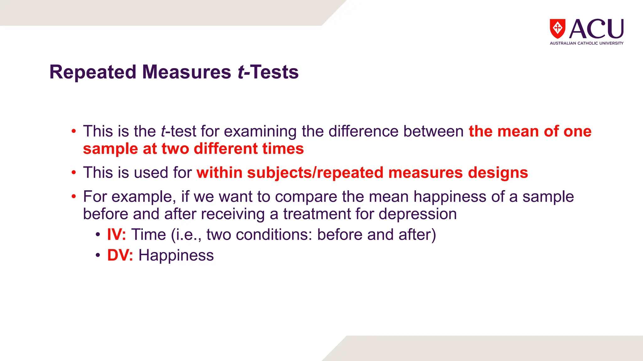
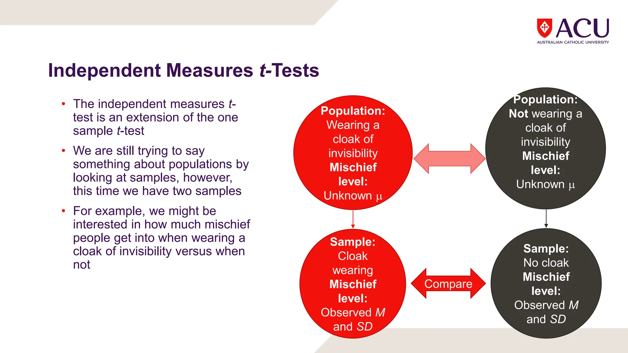
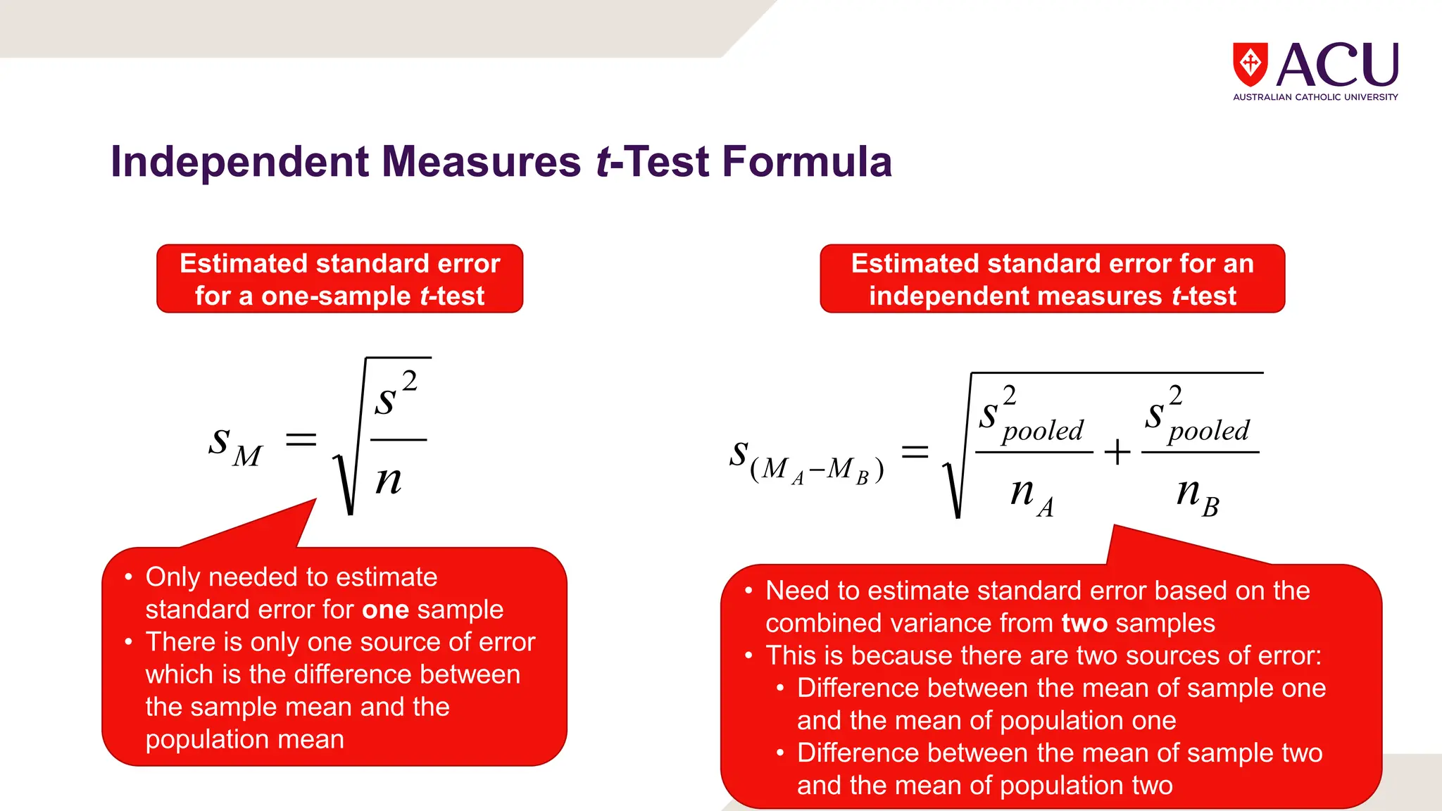
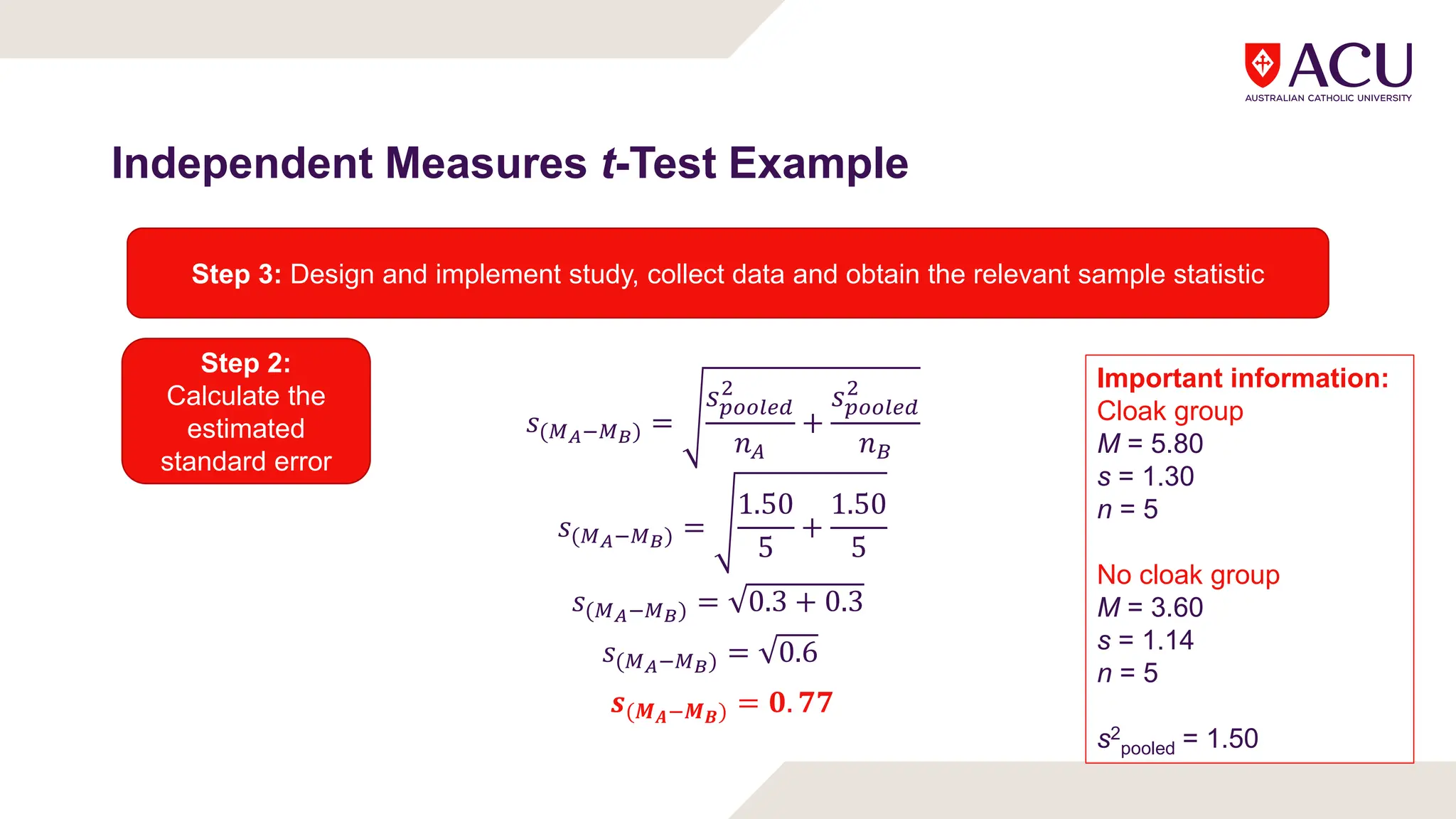
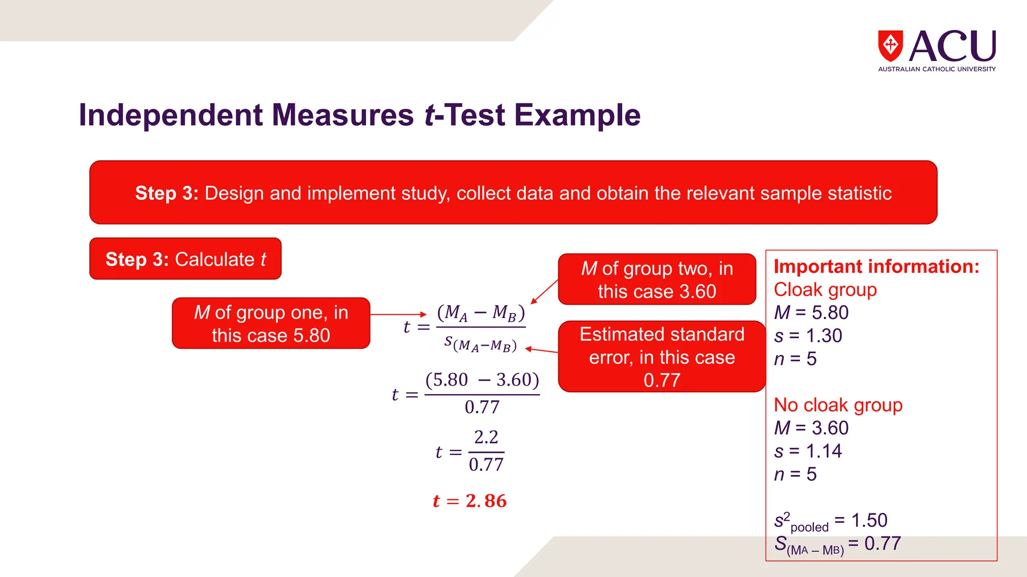
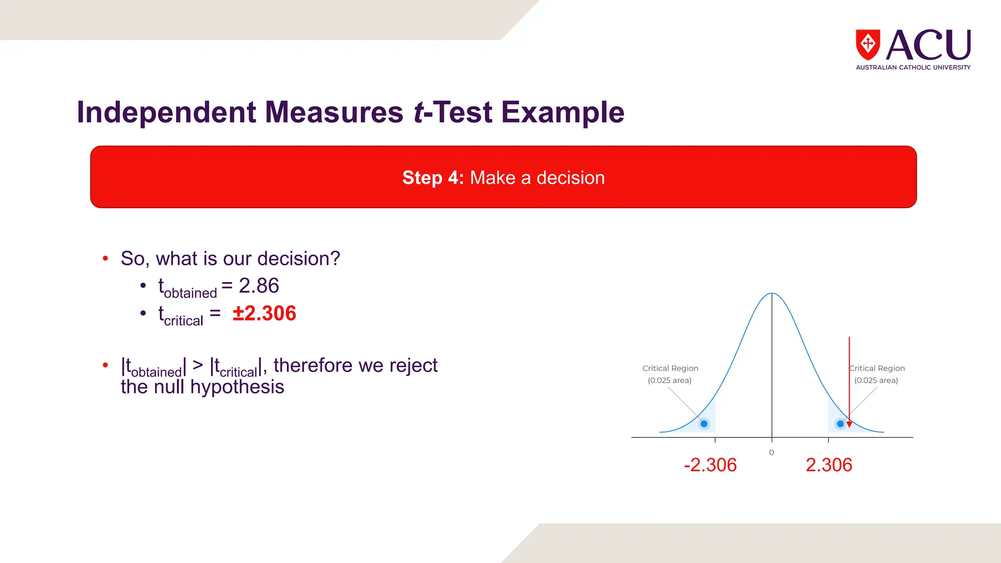
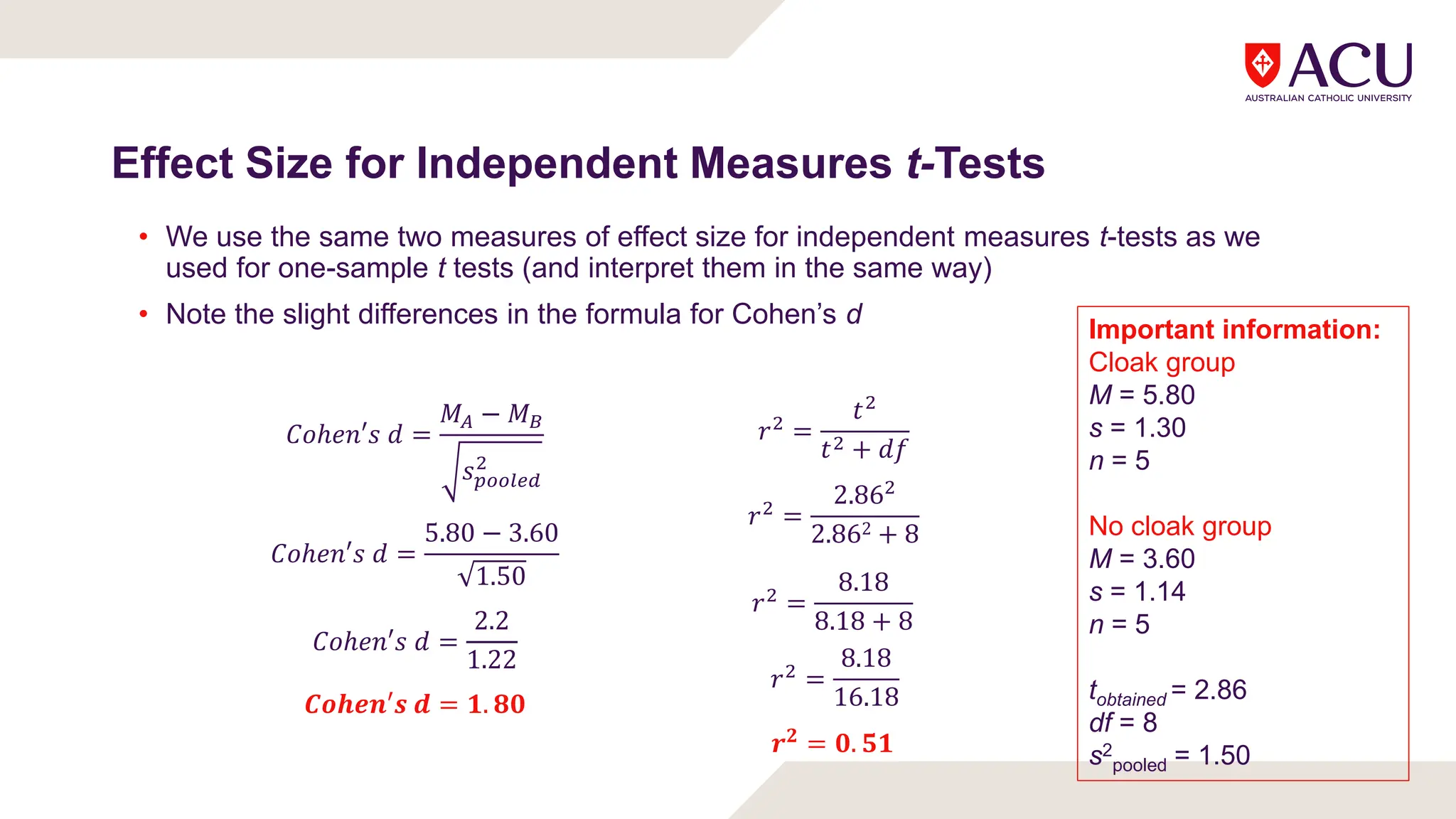
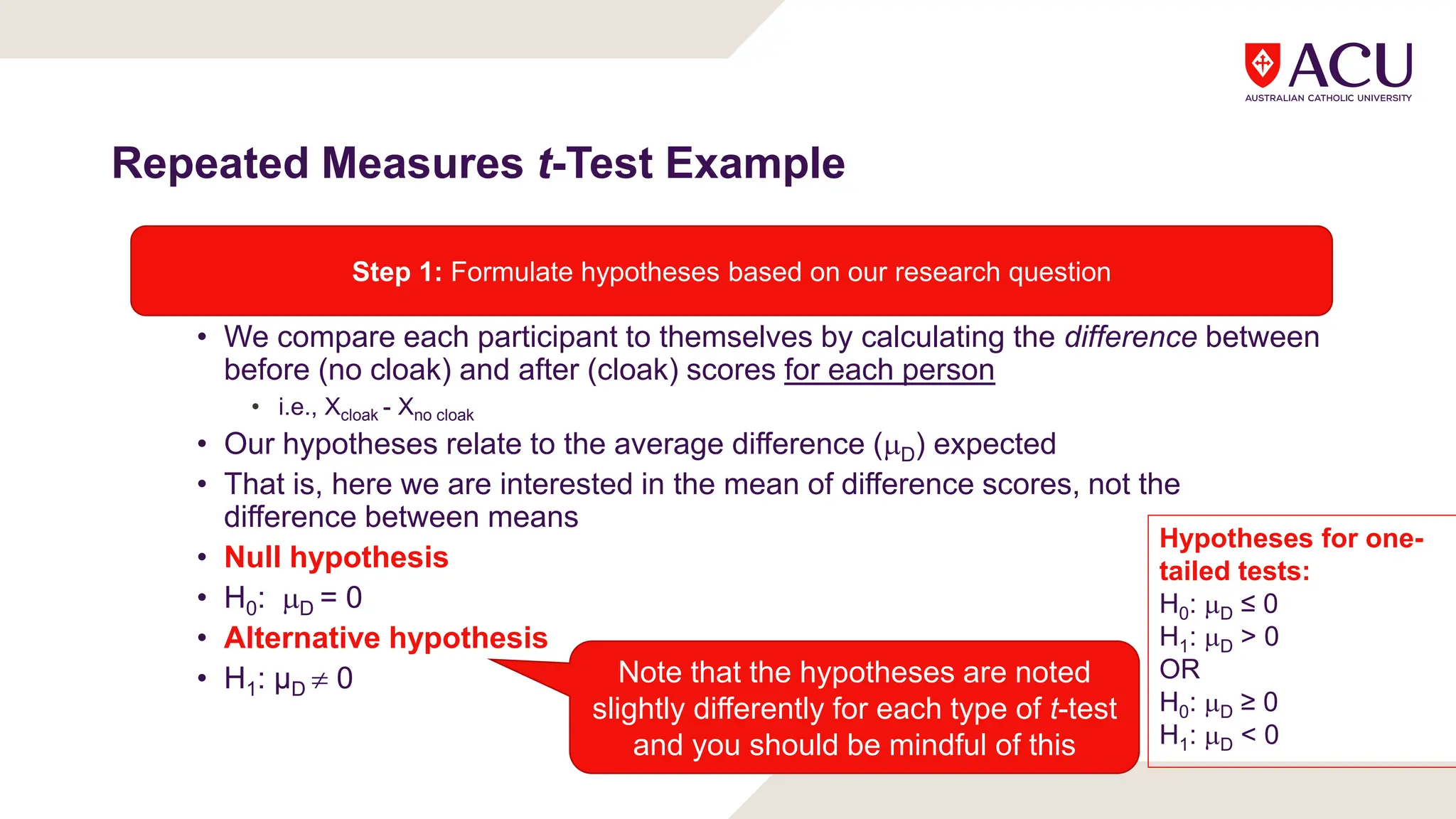
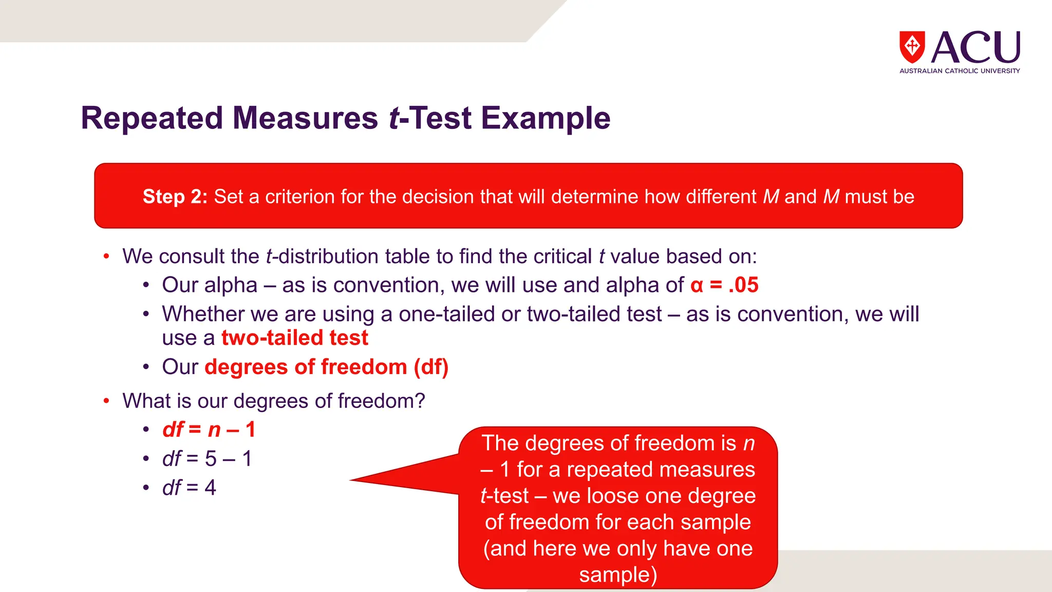
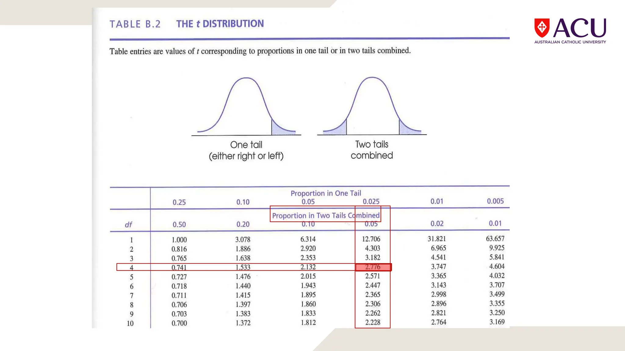
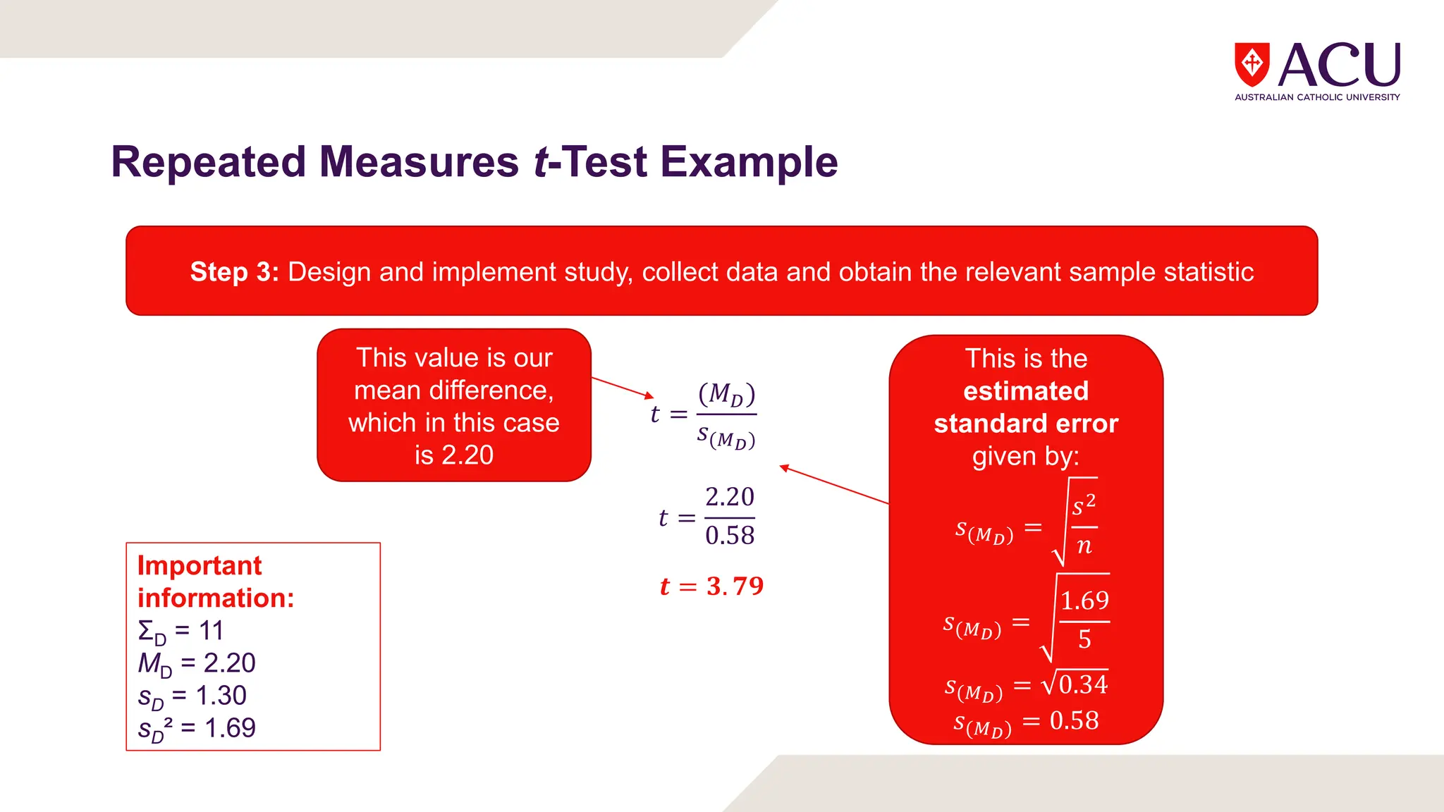
Introduction to Statistics: Types of T-Tests

Types of t-Tests
• There are three types of t-tests that we use in different scenarios:
• One-sample t-test
• Compares mean of one sample to a population mean
• Independent measures t-test
• Compares mean of one sample to the mean of another sample
• Repeated measures t-test
• Compares mean of one sample at one time point to the mean of
the same sample at another time point

Types of Research Designs
REPEATED MEASURES/WITHIN
SUBJECTS DESIGNS
• The same group of participants is
administered different “levels” of the IV at
different times
Group of people who get chocolate at one time point
and no chocolate at another
INDEPENDENT
GROUPS/BETWEEN GROUPS
DESIGNS
• Different groups of participants are
administered different “levels” of the IV
(participants are randomly assigned to
groups)
No chocolate group Chocolate group

Independent Measures t-Tests
• This is the t-test for examining the difference between two separate sample
means
• This is used for independent groups/between subjects designs
• For example, if we want to compare the mean happiness of those who were
given a treatment for depression to those who were not given a treatment for
depression
• IV: Treatment group (two groups: either treatment or control)
• DV: Happiness

Repeated Measures t-Tests
• This is the t-test for examining the difference between the mean of one
sample at two different times
• This is used for within subjects/repeated measures designs
• For example, if we want to compare the mean happiness of a sample
before and after receiving a treatment for depression
• IV: Time (i.e., two conditions: before and after)
• DV: Happiness

Independent Measures t-Tests
• The independent measures t-
test is an extension of the one
sample t-test
• We are still trying to say
something about populations by
looking at samples, however,
this time we have two samples
• For example, we might be
interested in how much mischief
people get into when wearing a
cloak of invisibility versus when
not
Population:
Wearing a
cloak of
invisibility
Mischief
level:
Unknown 
Sample:
Cloak
wearing
Mischief
level:
Observed M
and SD
Population:
Not wearing a
cloak of
invisibility
Mischief
level:
Unknown 
Sample:
No cloak
Mischief
level:
Observed M
and SD
Compare

Independent Measures t-Test Formula
• Independent measures t-tests are about differences between means
• In fact, logically:
t =
( )
( . ., )
)
(
)
(
)
(
B
A M
M
B
A
B
A
s
M
M
t







The observed difference
between the sample means
The hypothesised
difference between the
population means under H0
Estimated standard error
(for the difference between
the means)

)
(
)
(
)
(
B
A M
M
B
A
B
A
s
M
M
t







The observed difference
between the sample means
The hypothesised
difference between the
population means under H0
(for the difference between
the means)
Under the null
hypothesis, this will
always equal zero, so we
will simplify our formula
by removing it

• Just like the one-sample t-test, you can see that we are using sample statistics as a way to
estimate population parameters
)
(
)
(
B
A M
M
B
A
s
M
M
t



The mean difference
between the two samples
• Mean of sample A (mischief
with cloak) minus mean of
sample B (mischief without
cloak)
• Average distance (expected due to
sampling error alone) between two
sample means under the null
hypothesis
• Estimated based on sample
information

B
pooled
A
pooled
M
M
n
s
n
s
s B
A
2
2
)
( 


)
(
)
(
B
A M
M
B
A
s
M
M
t



•The calculation of estimated
standard error uses this
formula
•This accounts for the fact
that there are two sources of
error now: MA approximates
μA with some error and MB
approximates μB with some
error

B
pooled
A
pooled
M
M
n
s
n
s
s B
A
2
2
)
( 


n
s
sM
2

for a one-sample t-test
Estimated standard error for an
independent measures t-test
• Only needed to estimate
standard error for one sample
• There is only one source of error
which is the difference between
the sample mean and the
population mean
• Need to estimate standard error based on the
combined variance from two samples
• This is because there are two sources of error:
• Difference between the mean of sample one
and the mean of population one
• Difference between the mean of sample two
and the mean of population two

Pooled variance
B
pooled
A
pooled
M
M
n
s
n
s
s B
A
2
2
)
( 


•The s2
pooled combines the two sample variances into a single value called
the pooled variance
•If the sample sizes are equal, s2
pooled is simply the average variance
across the two samples. That is:
s2
pooled =

Pooled variance
B
pooled
A
pooled
M
M
n
s
n
s
s B
A
2
2
)
( 


•However, when our sample sizes are unequal, the larger sample is better able to
estimate the variance of the population – so we should rely on that more (i.e., we
should weight it more heavily)
•Therefore, when sample sizes are not equal, one these formulas for the pooled
variance are used:
•You need to know these exist and why, however, you don’t need to understand
the complex calculation of pooled variance with unequal sample sizes for
PSYC104
B
A
B
B
A
A
pooled
B
A
B
A
pooled
df
df
s
df
s
df
s
df
df
SS
SS
s






2
2
2
2
;

Independent Measures t-Test Example
• Let’s go back to our invisibility cloak example
• Our research question is: Is there a difference in mischievous
behaviour between those who wear a cloak of visibility versus those
who do not?
• We recruit 10 people and randomly assign them to one of two groups:
• Cloak group: wears the invisibility cloak
• No cloak group: does not wear the invisibility cloak
• We observe them for an hour and rate their mischievousness on a
scale of 0 (no mischief) – 10 (lots of mischief)

Participant
ID
Group Mischief
(/10)
1 Cloak 7
2 Cloak 6
3 Cloak 7
4 Cloak 5
5 Cloak 4
6 No Cloak 4
7 No Cloak 3
8 No Cloak 5
9 No Cloak 2
10 No Cloak 4
Important information:
Cloak group
M = 5.80
s = 1.30
n = 5
No cloak group
M = 3.60
s = 1.14
n = 5

• It is a four-step process:
1. Generate hypotheses (H0 and H1)
2. Select critical region
3. Gather data, compute statistic – this time using our new formula
for t
4. Make a decision
• If the obtained statistic is in the critical region – reject the null hypothesis
• If the obtained statistic is not in the critical region – fail to reject the null hypothesis

• The hypotheses are about the difference between (population)
means from each group
• i.e., cloak - no cloak
• hypothesis
• H0: cloak - no cloak = 0 OR H0: cloak = no cloak
• Alternative hypothesis
• H1: cloak - no cloak  0 OR H1: cloak ≠ no cloak
Step 1: Formulate hypotheses based on our research question
Hypotheses for one-tailed
tests:
H0: cloak- no cloak ≤ 0
H1: cloak- no cloak > 0
OR
H0: cloak- no cloak ≥ 0
H1: cloak- no cloak < 0

• We consult the t-distribution table to find the critical t value based on:
• Our alpha – as is convention, we will use and alpha of α = .05
• Whether we are using a one-tailed or two-tailed test – as is convention, we will
use a two-tailed test
• Our degrees of freedom (df)
• What is our degrees of freedom?
• df = n – 2
• df = 10 – 2
• df = 8
Step 2: Set a criterion for the decision that will determine how different M and M must be
The degrees of freedom is n
– 2 for an independent
measures t-test – we loose
one degree of freedom for
each sample

B
pooled
A
pooled
M
M
n
s
n
s
s B
A
2
2
)
( 


Step 3: Design and implement study, collect data and obtain the relevant sample statistic
𝑡 =
(𝑀 − 𝑀 )
𝑠( )
Step 1:
Calculate
the pooled
variance
Step 2:
Calculate the
estimated
standard error
Step 3: Calculate
t

Step 1:
Calculate
the pooled
variance
Important
information:
Cloak group
M = 5.80
s = 1.30
n = 5
No cloak group
M = 3.60
s = 1.14
n = 5
s2
pooled =
s2
pooled =
. ( . )
s2
pooled =
. .
s2
pooled =
.
s2
pooled = 1.50

Cloak group
M = 5.80
s = 1.30
n = 5
No cloak group
M = 3.60
s = 1.14
n = 5
s2
pooled = 1.50
Step 2:
Calculate the
estimated
standard error
𝑠( ) =
𝑠
𝑛
+
𝑠
𝑛
𝑠( ) =
1.50
5
+
1.50
5
𝑠( ) = 0.3 + 0.3
𝑠( ) = 0.6
𝒔(𝑴𝑨 𝑴𝑩) = 𝟎. 𝟕𝟕

Step 3: Calculate t
𝑡 =
(𝑀 − 𝑀 )
𝑠( )
M of group one, in
this case 5.80
M of group two, in
this case 3.60
Estimated standard
error, in this case
0.77
𝑡 =
(5.80 − 3.60)
0.77
𝑡 =
2.2
0.77
𝒕 = 𝟐. 𝟖𝟔
Cloak group
M = 5.80
s = 1.30
n = 5
No cloak group
M = 3.60
s = 1.14
n = 5
s2
pooled = 1.50
S(MA – MB) = 0.77

• So, what is our decision?
• tobtained = 2.86
• tcritical = ±2.306
• |tobtained| > |tcritical|, therefore we reject
the null hypothesis
Step 4: Make a decision
-2.306 2.306

Effect Size for Independent Measures t-Tests
• We use the same two measures of effect size for independent measures t-tests as we
used for one-sample t tests (and interpret them in the same way)
• Note the slight differences in the formula for Cohen’s d
𝐶𝑜ℎ𝑒𝑛′𝑠 𝑑 =
𝑀 − 𝑀
𝑠
𝑟 =
𝑡
𝑡 + 𝑑𝑓
5.80 − 3.60
1.50
Cloak group
M = 5.80
s = 1.30
n = 5
No cloak group
M = 3.60
s = 1.14
n = 5
tobtained = 2.86
df = 8
s2
pooled = 1.50
2.2
1.22
𝑪𝒐𝒉𝒆𝒏′𝒔 𝒅 = 𝟏. 𝟖𝟎
𝑟 =
2.86
2.862 + 8
𝑟 =
8.18
8.18 + 8
𝑟 =
8.18
16.18
𝒓𝟐 = 𝟎. 𝟓𝟏

Assumptions of Independent Measures t-Tests
• Design-based assumptions:
• Random sampling
• Observations within each group should be independent of each other
• Interval or ratio scale of measurement for the dependent variable
• Data-based assumptions:
• The dependent variable should be normally distributed within each group
• Robust to violations of this assumption when n > 30
• Homogeneity of variances
• The variances of the groups should be roughly equal
• SPSS checks this automatically and gives you an alternative if this assumption
is violated

Normality
•We assess that the dependent variable (i.e., mischievousness) is normally distributed in
each group (i.e., cloak and no cloak)
•We want the data to be normal in terms of its skew and kurtosis

Homogeneity of Variances
• We require the variances of the two populations to be relatively equal

Repeated Measures t-Tests
• Repeated measures/within subjects research designs compare each
participant to themselves
• When you compare a participant to themselves, you can “partial out” or
“remove” individual differences factors as an explanation for the
differences between the two measurement times
• Repeated measures designs require a different statistic – the repeated
measures t-test

Repeated Measures t-Test Formula
)
(
)
(
)
(
D
M
D
D
s
M
t



Mean of the
difference scores in
your sample
Mean difference in
population between
time one and time two
under H0
𝑠( ) =
𝑠
𝑛
• Here we are interested in
the variance of the
difference scores
Under the null
hypothesis, this will
always equal zero, so
we will simplify our
formula by removing it
You will sometimes
see the formula
written without the
subscript “D” which
means “difference” –
but it means the
same thing

Repeated Measures t-Test Example
• Let’s go back to our invisibility cloak example (but change it slightly)
• Our research question is: Is there a difference in the amount of
mischief people get up to when they wear a cloak of visibility versus
when they do not?
• We recruit 5 people and have them undergo two conditions
• Cloak condition: wear the invisibility cloak
• No cloak condition: do not wear the invisibility cloak
• We observe them for an hour in each condition and rate their
mischievousness on a scale of 0 (no mischief) – 10 (lots of mischief)

Participant
ID
Mischief using
cloak
(after cloak)
Mischief not
using cloak
(before cloak)
1 7 4
2 6 3
3 7 5
4 5 2
5 4 4

• It is a four step process:
1. Generate hypotheses (H0 and H1)
2. Select critical region
3. Gather data, compute statistic – this time using our new formula
for t
4. Make a decision
• If the obtained statistic is in the critical region – reject the null hypothesis
• If the obtained statistic is not in the critical region – fail to reject the null hypothesis

• We compare each participant to themselves by calculating the difference between
before (no cloak) and after (cloak) scores for each person
• i.e., Xcloak - Xno cloak
• Our hypotheses relate to the average difference (D) expected
• That is, here we are interested in the mean of difference scores, not the
difference between means
• Null hypothesis
• H0: D = 0
• Alternative hypothesis
• H1: µD  0
Step 1: Formulate hypotheses based on our research question
Note that the hypotheses are noted
slightly differently for each type of t-test
and you should be mindful of this
Hypotheses for one-
tailed tests:
H0: D ≤ 0
H1: D > 0
OR
H0: D ≥ 0
H1: D < 0

• We consult the t-distribution table to find the critical t value based on:
• Our alpha – as is convention, we will use and alpha of α = .05
• Whether we are using a one-tailed or two-tailed test – as is convention, we will
use a two-tailed test
• Our degrees of freedom (df)
• What is our degrees of freedom?
• df = n – 1
• df = 5 – 1
• df = 4
Step 2: Set a criterion for the decision that will determine how different M and M must be
The degrees of freedom is n
– 1 for a repeated measures
t-test – we loose one degree
of freedom for each sample
(and here we only have one
sample)

• We start by calculating difference scores between before and after for each participant
• We then determine the mean (MD), variance and standard deviation of these scores
Important
information:
ƩD = 11
MD = 2.20
sD = 1.30
sD² = 1.69
Participant
ID
Mischief using
cloak
(after cloak)
Mischief not
using cloak
(before cloak)
1 7 4
2 6 3
3 7 5
4 5 2
5 4 4
Participant
ID
Mischief using
cloak
(after cloak)
Mischief not
using cloak
(before cloak)
Difference (after – before)
1 7 4 7 – 4 = 3
2 6 3 6 – 3 = 3
3 7 5 7 – 5 = 2
4 5 2 5 – 2 = 3
5 4 4 4 – 4 = 0

This value is our
mean difference,
which in this case
is 2.20
This is the
estimated
standard error
given by:
𝑠( ) =
𝑠
𝑛
𝑠( ) =
1.69
5
𝑠( ) = 0.34
𝑠( ) = 0.58
𝑡 =
2.20
0.58
𝒕 = 𝟑. 𝟕𝟗
𝑡 =
(𝑀 )
𝑠( )
Important
information:
ƩD = 11
MD = 2.20
sD = 1.30
sD² = 1.69

• So, what is our decision?
• tobtained = 3.79
• tcritical = ±2.776
• |tobtained| > |tcritical|, therefore we reject
the null hypothesis
Step 4: Make a decision
-2.776 2.776

Effect Size for Repeated Measures t-Tests
• We use the same two measures of effect size for repeated measures t-tests as we used
for one-sample t tests and independent measures t-test (and interpret them in the same
way)
• Note the slight differences in the formula for Cohen’s d
𝑟 =
𝑡
𝑡 + 𝑑𝑓
2.20
1.30
𝑪𝒐𝒉𝒆𝒏 𝒔 𝒅 = 𝟏. 𝟔𝟗
𝑟 =
3.79
3.792 + 4
𝑟 =
14.36
14.36 + 4
𝑟 =
14.36
18.36
𝑀
𝑠𝐷
Important
information:
ƩD = 11
MD = 2.20
sD = 1.30
sD² = 1.69
tobtained = 3.79
df = 4
𝑟 = 0.78

Assumptions of Repeated Measures t-Tests
• Design-based assumptions:
• Observations within each treatment condition should be independent
• Interval or ratio scale of measurement for the dependent variable
• Data-based assumptions:
• Normality of difference scores
• Robust to violations of this assumption when n > 30

Other Uses for Repeated Measures t-Tests
• We can also use a repeated measures t-test for a matched subjects research
design
• Recall that this is a research design where we don’t have the same people
tested twice, but pairs of participants who have been matched with each other
based on important control variable(s)
• e.g., match two participants in terms of age, sex and IQ and put one in Group A and one in
Group B
• Because participants have been carefully matched, we can treat them as if
they are the same person and use the repeated measure t-test

Introduction to Statistics: Types of T-Tests

More Related Content

Similar to Introduction to Statistics: Types of T-Tests

Recently uploaded

Introduction to Statistics: Types of T-Tests