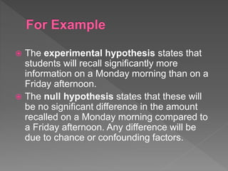
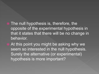
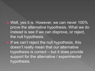
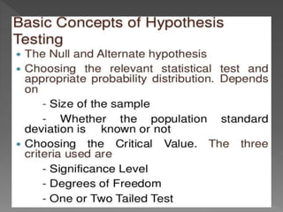
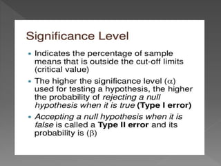
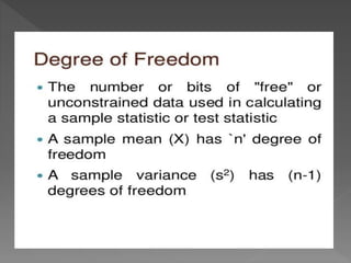
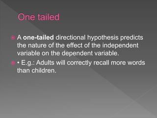
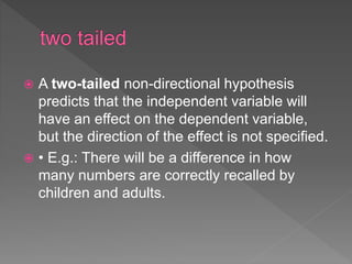
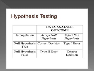
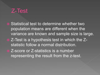
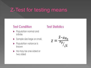
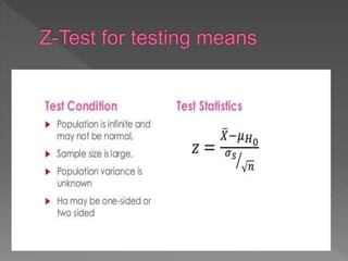
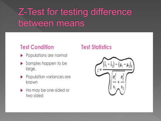
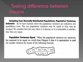
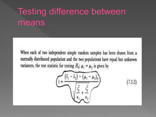
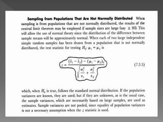
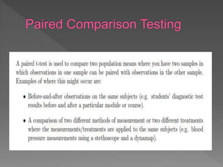
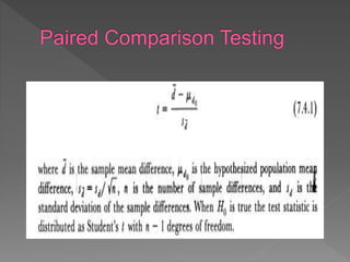
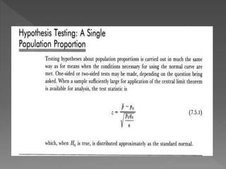
BUS 308 Week 3 Lecture 1 Examining Differences - Continued.docxcurwenmichaela
BUS 308 Week 3 Lecture 1
Examining Differences - Continued
Expected Outcomes
After reading this lecture, the student should be familiar with:
1. Issues around multiple testing
2. The basics of the Analysis of Variance test
3. Determining significant differences between group means
4. The basics of the Chi Square Distribution.
Overview
Last week, we found out ways to examine differences between a measure taken on two
groups (two-sample test situation) as well as comparing that measure to a standard (a one-sample
test situation). We looked at the F test which let us test for variance equality. We also looked at
the t-test which focused on testing for mean equality. We noted that the t-test had three distinct
versions, one for groups that had equal variances, one for groups that had unequal variances, and
one for data that was paired (two measures on the same subject, such as salary and midpoint for
each employee). We also looked at how the 2-sample unequal t-test could be used to use Excel
to perform a one-sample mean test against a standard or constant value. This week we expand
our tool kit to let us compare multiple groups for similar mean values.
A second tool will let us look at how data values are distributed – if graphed, would they
look the same? Different shapes or patterns often means the data sets differ in significant ways
that can help explain results.
Multiple Groups
As interesting as comparing two groups is, often it is a bit limiting as to what it tells us.
One obvious issue that we are missing in the comparisons made last week was equal work. This
idea is still somewhat hard to get a clear handle on. Typically, as we look at this issue, questions
arise about things such as performance appraisal ratings, education distribution, seniority impact,
etc.
Some of these can be tested with the tools introduced last week. We can see, for
example, if the performance rating average is the same for each gender. What we couldn’t do, at
this point however, is see if performance ratings differ by grade, do the more senior workers
perform relatively better? Is there a difference between ratings for each gender by grade level?
The same questions can be asked about seniority impact. This week will give us tools to expand
how we look at the clues hidden within the data set about equal pay for equal work.
ANOVA
So, let’s start taking a look at these questions. The first tool for this week is the Analysis
of Variance – ANOVA for short. ANOVA is often confusing for students; it says it analyzes
variance (which it does) but the purpose of an ANOVA test is to determine if the means of
different groups are the same! Now, so far, we have considered means and variance to be two
distinct characteristics of data sets; characteristics that are not related, yet here we are saying that
looking at one will give us insight into the other.
The reason is due to the way the variance is an.
When you are working on the Inferential Statistics Paper I want yo.docxalanfhall8953
When you are working on the Inferential Statistics Paper I want you to format your paper with the following information
I. Introduction – What are inferential statistics and what is the research problem and hypothesis of the article?
II. Methods – Who are the subjects and variables within the article?
III. Results – What is the statistical analysis used, why were these tests chosen? What were the results of these tests and what do they mean?
IV. Discussion – What were the strengths of this article? What would you have done differently in terms of variables and statistical analysis? Why?
V. Conclusion – Reiterate the introduction and include relevant information that answers the questions regarding the hypothesis.
`
Read: Chapter 3 and 4 of Statistics for the Behavioral and Social Sciences.
Participate in One discussion.
Discussion 1 –Standard Normal Distribution– This allows you to look at any data set into the standard distribution form.
Quiz – Hypothesis testing
Submit your Inferential Statics Article Critique – Read Differential Effects of a Body Image Exposure Session on Smoking Urge Between Physically Active and Sedentary Female Smokers. What is the research question and hypothesis? Identify what variables were present, what inferential statistics were used and why, and if proper research methods were used. See grading rubric for full details.
Discussion Post Expectations:
Your initial post (your answer) is due by Day 3 (Thursday) of this week for Discussion 1.
When grading the Standard Normative Distribution discussion I will be looking for your answer to contain:
Week 2 Discussion 1 Board Rubric
Earned
Weight
Content Criteria
0.5
Student identifies and defines what Standard Normative Distribution (SND) is.
Student explains why it is needed to use a SND to compare two data sets.
0.5
Student identifies the purpose of a z-score in a SND.
0.5
Student identifies the purpose of a percentage in a SND.
0.25
Student explains whether a z-score or a percentage does a better job of identifying proportion of a SND.
0.25
The student responds to at least two classmates’ initial posts by Day 7.
1
Student uses correct spelling, grammar and sentence structure.
2
5
Grading - The discussions are both worth a total of 5 points. The breakdown of the grading for this week’s assignment (per discussion assignment) will be as follows:
Posting your answer by the due date (Day 3, Thursday) is worth 4 points. These five points will be based on the information outlined within the Discussion Assignment Expectations. Content will be worth 2 points and format; spelling and grammar will be worth 2 points.
Responding to two of your classmates (for each assignment) is worth 1 point. The answers must be substantive and go beyond “I agree” or “Good job” to qualify for this point.
Intellectual Elaboration:
In Wee.
Week 6 DQ1. What is your research questionIs there a differen.docxcockekeshia
Week 6 DQ
1. What is your research question?
Is there a difference between the math utility of a male and a female?
2. What is the null hypothesis for your question?
Hn There is no difference in the math utility between male and female.
Alternative hypotheses can also be created in the case the null hypothesis is proven incorrect. Two alternative hypotheses are:
Ha1 Feales have a higher math utility.
Ha2 Males have a higher math utility.
3. What research design would align with this question?
According to Frankfort-Nachmias and Leon-Guerrero (2015) a descriptive research design would be best for this type of study.
4. What comparison of means test was used to answer the question (be sure to defend the use of the test using the article you found in your search)?
The independent-samples T test was used to analyze the means for this data.
5. What dependent variable was used and how is it measured?
The dependent variable is the student’s math utility. It is measured from -3.51 to 1.31(University high school longitudinal study dataset. (2009).
6. What independent variable is used and how is it measured?
Either male (1) of female (2) (University high school longitudinal study dataset. (2009).
7. If you found significance, what is the strength of the effect?
The significance was 0.0000. This is much better than the standard of .05 significance as outlined by Frankfort-Nachmias and Leon-Guerrero (2015).
8. Identify your research question and explain your results for a lay audience, what is the answer to your research question?
My research question was “Is there a difference between the math utility of a male and a female?” Based on the analysis of the means (or average) through testing using the independent-samples T test there was no measurable difference between the math utility of male or females. This leads us to accept the null hypothesis of “There is no difference in the math utility between male and female” as true.
Group Statistics
T1 Student's sex
N
Mean
Std. Deviation
Std. Error Mean
T1 Scale of student's mathematics utility
Male
9453
.0140
1.01962
.01049
Female
9349
-.0481
.97291
.01006
Independent Samples Test
Levene's Test for Equality of Variances
t-test for Equality of Means
F
Sig.
t
df
Sig. (2-tailed)
Mean Difference
Std. Error Difference
95% Confidence Interval of the Difference
Lower
Upper
T1 Scale of student's mathematics utility
Equal variances assumed
17.400
.000
4.276
18800
.000
.06216
.01454
.03367
.09066
Equal variances not assumed
4.277
18775.932
.000
.06216
.01453
.03367
.09065
University high school longitudinal study dataset. (2009).
References
Frankfort-Nachmias, C., & Leon-Guerrero, A. (2015). Social statistics for a diverse society (7th ed.). Thousand Oaks, CA: Sage Publications.
University high school longitudinal study dataset. (2009). Retrieved from class.waldenu.edu
The t Test for Related Samples
Program Transcript
MAT.
Assessment 3 ContextYou will review the theory, logic, and a.docxgalerussel59292
Assessment 3 Context
You will review the theory, logic, and application of t-tests. The t-test is a basic inferential statistic often reported in psychological research. You will discover that t-tests, as well as analysis of variance (ANOVA), compare group means on some quantitative outcome variable.
Recall that null hypothesis tests are of two types: (1) differences between group means and (2) association between variables. In both cases there is a null hypothesis and an alternative hypothesis. In the group means test, the null hypothesis is that the two groups have equal means, and the alternative hypothesis is that the two groups do not have equal means. In the association between variables type of test, the null hypothesis is that the correlation coefficient between the two variables is zero, and the alternative hypothesis is that the correlation coefficient is not zero.
Notice in each case that the hypotheses are mutually exclusive. If the null is false, the alternative must be true. The purpose of null hypothesis statistical tests is generally to show that the null has a low probability of being true (the p value is less than .05) – low enough that the researcher can legitimately claim it is false. The reason this is done is to support the allegation that the alternative hypothesis is true.
In this context you will be studying the details of the first type of test. This is the test of difference between group means. In variations on this model, the two groups can actually be the same people under different conditions, or one of the groups may be assigned a fixed theoretical value. The main idea is that two mean values are being compared. The two groups each have an average score or mean on some variable. The null hypothesis is that the difference between the means is zero. The alternative hypothesis is that the difference between the means is not zero. Notice that if the null is false, the alternative must be true. It is first instructive to consider some of the details of groups. Means, and difference between them.
Null Hypothesis Significance Test
The most common forms of the Null Hypothesis Significance Test (NHST) are three types of t tests, and the test of significance of a correlation. The NHST also extends to more complex tests, such as ANOVA, which will be discussed separately. Below, the null hypothesis and the alternative hypothesis are given for each of the following tests. It would be a valuable use of your time to commit the information below to memory. Once this is done, then when we refer to the tests later, you will have some structure to make sense of the more detailed explanations.
1. One-sample t test: The question in this test is whether a single sample group mean is significantly different from some stated or fixed theoretical value - the fixed value is called a parameter.
· Null Hypothesis: The difference between the sample group mean and the fixed value is zero in the population.
· Alternative hypothesis: T.
BUS308 – Week 5 Lecture 1 A Different View Expected Ou.docxcurwenmichaela
BUS308 – Week 5 Lecture 1
A Different View
Expected Outcomes
After reading this lecture, the student should be familiar with:
1. What a confidence interval for a statistic is.
2. What a confidence interval for differences is.
3. The difference between statistical and practical significance.
4. The meaning of an Effect Size measure.
Overview
Years ago, a comedy show used to introduce new skits with the phrase “and now for
something completely different.” That seems appropriate for this week’s material.
This week we will look at evaluating our data results in somewhat different ways. One of
the criticisms of the hypothesis testing procedure is that it only shows one value, when it is
reasonably clear that a number of different values would also cause us to reject or not reject a
null hypothesis of no difference. Many managers and researchers would like to see what these
values could be; and, in particular, what are the extreme values as help in making decisions.
Confidence intervals will help us here.
The other criticism of the hypothesis testing procedure is that we can “manage” the
results, or ensure that we will reject the null, by manipulating the sample size. For example, if
we have a difference in a customer preference between two products of only 1%, is this a big
deal? Given the uncertainty contained in sample results, we might tend to think that we can
safely ignore this result. However, if we were to use a sample of, say, 10,000, we would find
that this difference is statistically significant. This, for many, seems to fly in the face of
reasonableness. We will look at a measure of “practical significance,” meaning the likelihood of
the difference being worth paying any attention to, called the effect size to help us here.
Confidence Intervals
A confidence interval is a range of values that, based upon the sample results, most likely
contains the actual population parameter. The “most likely” element is the level of confidence
attached to the interval, 95% confidence interval, 90% confidence interval, 99% confidence
interval, etc. They can be created at any time, with or without performing a statistical test, such
as the t-test.
A confidence interval may be expressed as a range (45 to 51% of the town’s population
support the proposal) or as a mean or proportion with a margin of error (48% of the town
supports the proposal, with a margin of error of 3%). This last format is frequently seen with
opinion poll results, and simply means that you should add and subtract this margin of error from
the reported proportion to obtain the range. With either format, the confidence percent should
also be provided.
Confidence intervals for a single mean (or proportion) are fairly straightforward to
understand, and relate to t-test outcomes simply. Details on how to construct the interval will be
given in this week’s second lecture. We want to understand how to interpret and understa.
STATISTICS : Changing the way we do: Hypothesis testing, effect size, power, ...Musfera Nara Vadia
STATISTICS : Changing the way we do: Hypothesis testing, effect size, power, confidence interval, two-tailed and one tailed test, and other misunderstood issues.
This lecture will help Research scholars at the starting of their research issues regarding definitions of variables, what is theory and creating a sapling map..
06-04-2024 - NYC Tech Week - Discussion on Vector Databases, Unstructured Data and AI
Round table discussion of vector databases, unstructured data, ai, big data, real-time, robots and Milvus.
A lively discussion with NJ Gen AI Meetup Lead, Prasad and Procure.FYI's Co-Found
Levelwise PageRank with Loop-Based Dead End Handling Strategy : SHORT REPORT ...Subhajit Sahu
Abstract — Levelwise PageRank is an alternative method of PageRank computation which decomposes the input graph into a directed acyclic block-graph of strongly connected components, and processes them in topological order, one level at a time. This enables calculation for ranks in a distributed fashion without per-iteration communication, unlike the standard method where all vertices are processed in each iteration. It however comes with a precondition of the absence of dead ends in the input graph. Here, the native non-distributed performance of Levelwise PageRank was compared against Monolithic PageRank on a CPU as well as a GPU. To ensure a fair comparison, Monolithic PageRank was also performed on a graph where vertices were split by components. Results indicate that Levelwise PageRank is about as fast as Monolithic PageRank on the CPU, but quite a bit slower on the GPU. Slowdown on the GPU is likely caused by a large submission of small workloads, and expected to be non-issue when the computation is performed on massive graphs.
Enhanced Enterprise Intelligence with your personal AI Data Copilot.pdfGetInData
Recently we have observed the rise of open-source Large Language Models (LLMs) that are community-driven or developed by the AI market leaders, such as Meta (Llama3), Databricks (DBRX) and Snowflake (Arctic). On the other hand, there is a growth in interest in specialized, carefully fine-tuned yet relatively small models that can efficiently assist programmers in day-to-day tasks. Finally, Retrieval-Augmented Generation (RAG) architectures have gained a lot of traction as the preferred approach for LLMs context and prompt augmentation for building conversational SQL data copilots, code copilots and chatbots.
In this presentation, we will show how we built upon these three concepts a robust Data Copilot that can help to democratize access to company data assets and boost performance of everyone working with data platforms.
Why do we need yet another (open-source ) Copilot?
How can we build one?
Architecture and evaluation
06-04-2024 - NYC Tech Week - Discussion on Vector Databases, Unstructured Data and AI
Discussion on Vector Databases, Unstructured Data and AI
https://www.meetup.com/unstructured-data-meetup-new-york/
This meetup is for people working in unstructured data. Speakers will come present about related topics such as vector databases, LLMs, and managing data at scale. The intended audience of this group includes roles like machine learning engineers, data scientists, data engineers, software engineers, and PMs.This meetup was formerly Milvus Meetup, and is sponsored by Zilliz maintainers of Milvus.
Analysis insight about a Flyball dog competition team's performanceroli9797
Insight of my analysis about a Flyball dog competition team's last year performance. Find more: https://github.com/rolandnagy-ds/flyball_race_analysis/tree/main
The Building Blocks of QuestDB, a Time Series Databasejavier ramirez
Talk Delivered at Valencia Codes Meetup 2024-06.
Traditionally, databases have treated timestamps just as another data type. However, when performing real-time analytics, timestamps should be first class citizens and we need rich time semantics to get the most out of our data. We also need to deal with ever growing datasets while keeping performant, which is as fun as it sounds.
It is no wonder time-series databases are now more popular than ever before. Join me in this session to learn about the internal architecture and building blocks of QuestDB, an open source time-series database designed for speed. We will also review a history of some of the changes we have gone over the past two years to deal with late and unordered data, non-blocking writes, read-replicas, or faster batch ingestion.
2. A hypothesis (plural hypotheses) is a
precise, testable statement of what the
researchers predict will be the outcome of
the study.
This usually involves proposing a possible
relationship between two variables: the
independent variable (what the researcher
changes) and the dependant variable (what
the research measures).
3. In research, there is a convention that the
hypothesis is written in two forms, the null
hypothesis, and the alternative hypothesis
(called the experimental hypothesis when
the method of investigation is an
experiment ).
Briefly, the hypotheses can be expressed in
the following ways:
4. The null hypothesis states that there is no
relationship between the two variables being
studied (one variable does not affect the
other). It states results are due to chance
and are not significant in terms of supporting
the idea being investigated.
5. The alternative hypothesis states that
there is a relationship between the two
variables being studied (one variable has an
effect on the other). It states that the results
are not due to chance and that they are
significant in terms of supporting the theory
being investigated.
6. In order to write the experimental and null
hypotheses for an investigation, you need to
identify the key variables in the study. A variable
is anything that can change or be changed, i.e.
anything which can vary. Examples of variables
are intelligence, gender, memory, ability, time
etc.
A good hypothesis is short and clear should
include the operationalized variables being
investigated.
7. Let’s consider a hypothesis that many
teachers might subscribe to: that students
work better on Monday morning than they do
on a Friday afternoon (IV=Day, DV=Standard
of work).
8. Now, if we decide to study this by giving the
same group of students a lesson on a
Monday morning and on a Friday afternoon
and then measuring their immediate recall
on the material covered in each session we
would end up with the following:
9. The experimental hypothesis states that
students will recall significantly more
information on a Monday morning than on a
Friday afternoon.
The null hypothesis states that these will
be no significant difference in the amount
recalled on a Monday morning compared to
a Friday afternoon. Any difference will be
due to chance or confounding factors.
10. The null hypothesis is, therefore, the
opposite of the experimental hypothesis in
that it states that there will be no change in
behavior.
At this point you might be asking why we
seem so interested in the null hypothesis.
Surely the alternative (or experimental)
hypothesis is more important?
11. Well, yes it is. However, we can never 100%
prove the alternative hypothesis. What we do
instead is see if we can disprove, or reject,
the null hypothesis.
If we can’t reject the null hypothesis, this
doesn’t really mean that our alternative
hypothesis is correct – but it does provide
support for the alternative / experimental
hypothesis.
12.
13.
14.
15. A one-tailed directional hypothesis predicts
the nature of the effect of the independent
variable on the dependent variable.
• E.g.: Adults will correctly recall more words
than children.
16. A two-tailed non-directional hypothesis
predicts that the independent variable will
have an effect on the dependent variable,
but the direction of the effect is not specified.
• E.g.: There will be a difference in how
many numbers are correctly recalled by
children and adults.
17.
18.
19.
20. Statistical test to determine whether two
population means are different when the
variance are known and sample size is large.
Z-Test is a hypothesis test in which the Z-
statistic follow a normal distribution.
Z-score or Z-statistics is a number
representing the result from the z-test.
21. A t-test is a type of inferential statistic used to
determine if there is a significant difference
between the means of two groups, which may
be related in certain features.
follows a normal distribution and may have
unknown variances.
Calculating a t-test requires three key data
values. They include the difference between the
mean values from each data set (called the
mean difference), the standard deviation of
each group, and the number of data values of
each group
22. There are three types of t-tests we can
perform based on the data at hand:
One sample t-test.
Independent two-sample t-test.
Paired sample t-test.
23. In a one-sample t-test, we compare the average (or
mean) of one group against the set average (or
mean). This set average can be any theoretical
value (or it can be the population mean).
Consider the following example – A research
scholar wants to determine if the average eating
time for a (standard size) burger differs from a set
value. Let’s say this value is 10 minutes. How do
you think the research scholar can go about
determining this?
He/she can broadly follow the below steps:
24. • Select a group of people
• Record the individual eating time of a standard size burger
• Calculate the average eating time for the group
• Finally, compare that average value with the set value of 10
• That, in a nutshell, is how we can perform a one-sample t-test.
Here’s the formula to calculate this:
where,
•t = t-statistic
•m = mean of the group
•µ = theoretical value or population mean
•s = standard deviation of the group
•n = group size or sample size
25. The two-sample t-test is used to compare the means of
two different samples.
Let’s say we want to compare the average height of the
male employees to the average height of the females.
Of course, the number of males and females should be
equal for this comparison. This is where a two-sample t-
test is used.
Here’s the formula to calculate the t-statistic for a two-
sample t-test:
•mA and mB are the means of two different samples
•nA and nB are the sample sizes
26. Here, the degree of freedom is nA + nB – 2.
We will follow the same logic we saw in a one-sample t-test to check if the
average of one group is significantly different from another group. That’s right –
we will compare the calculated t-statistic with the t-critical value.
•S2 is an estimator of the common variance of two samples, such as:
27. measure one group at two different times. We compare separate
means for a group at two different times or under two different
conditions.
For example, a certain manager realized that the productivity
level of his employees was trending significantly downwards. This
manager decided to conduct a training program for all his
employees with the aim of increasing their productivity levels.
How will the manager measure if the productivity levels
increased? It’s simple – just compare the productivity level of the
employees before versus after the training program.
Here, we are comparing the same sample (the employees) at two
different times (before and after the training). This is an example
of a paired t-test.
28. The formula to calculate the t-statistic for a
paired t-test is:
•t = t-statistic
•m = mean of the group
•µ = theoretical value or population mean
•s = standard deviation of the group
•n = group size or sample size