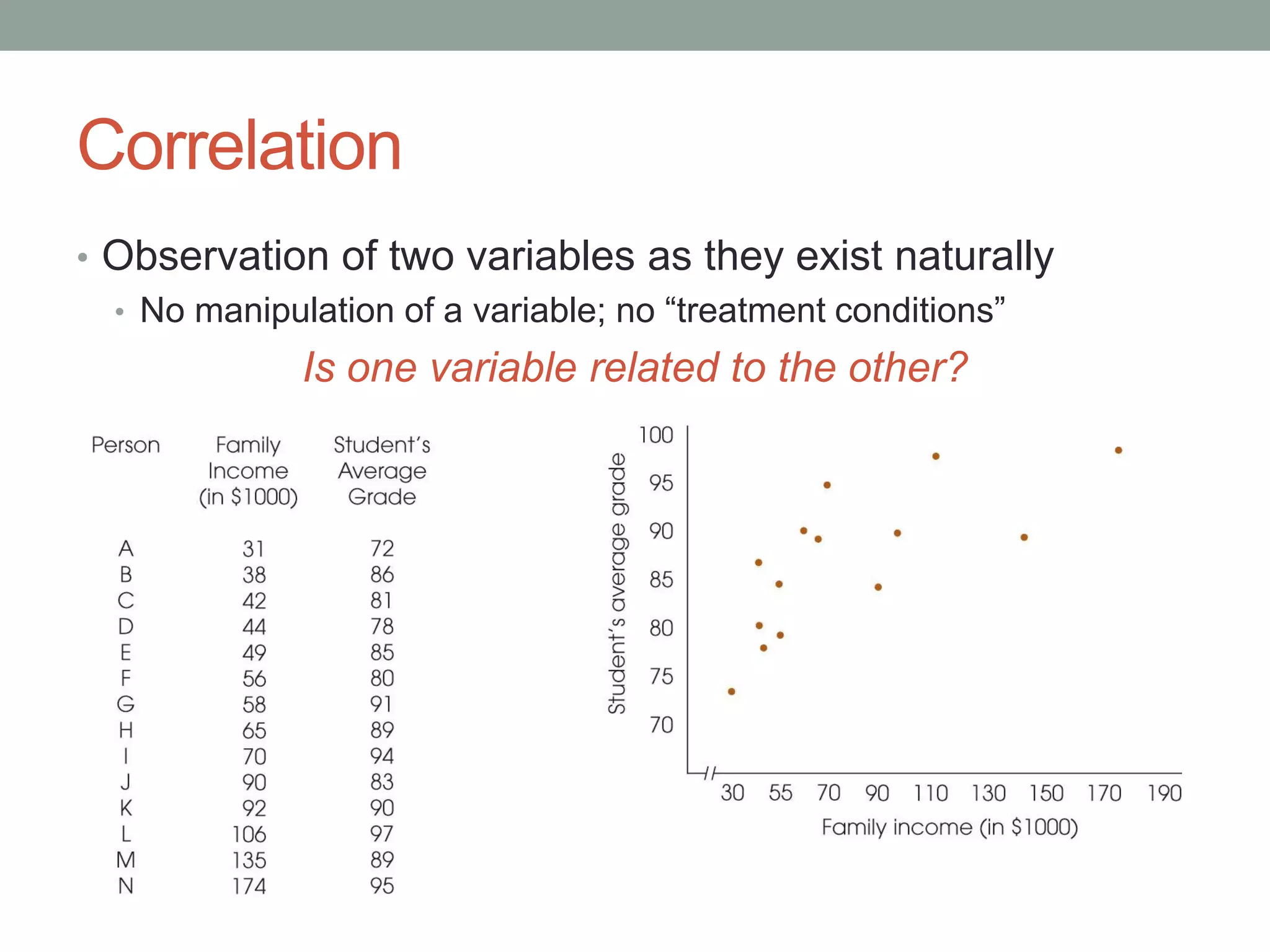
CHAPTER 15
Correlation
Gravetter &
Wallnau (ascitedintext)
• There is only one group of scores: Test scores
• Evaluating the mean of test scores will not tell us
anything
• We are now evaluating the relationship
between two variable
• How does is one variable related to the other?
Do students who
finish exams
quickly get
higher grades
than students
who take the
entire test time to
finish?
CHAPTER 15.1
Introduction
Correlation
• Observation of two variables as they exist naturally
• No manipulation of a variable; no “treatment conditions”
Is one variable related to the other?
The Characteristics of a Relationship
• The correlation describes three characteristics of the
relationship between two variables:
1. The direction (“+” or “-”)
Positive
(same direction)
Negative
(opposite direction)
The Characteristics of a Relationship
• The correlation describes three characteristics of the
relationship between two variables:
1. The direction
2. The form (linear vs. curvilinear)
The Characteristics of a Relationship
• The correlation describes three characteristics of the
relationship between two variables:
1. The direction
2. The form
3. The strength
• 0.01 (very weak) to .99 (very strong)
• 1.00 = perfect correlation
• 0.00 = no correlation
Strong
positive
correlation
Weak
negative
correlation
CHAPTER 15.2
The Pearson Correlation
Karl Pearson
3/27/1857 – 4/27/1936
The Pearson Correlation (r)
a.k.a The Pearson product-moment correlation
• Measures the degree and the direction of the linear
relationship between two variables
• It is also a ratio:
OR
separatelyvaryYandXwhichtodegree
thervary togeYandXwhichtodegreethe
r
separatelyYandXofyvariabilit
YandXofitycovariabilthe
r
Requirements for the Pearson r
• Each individual in the sample must have two scores, X
and Y
• All scores must be numerical values from an interval or
ratio scale of measurement
The Linear Relationship
• We are trying to determine if changes to one variable (X) is
accompanied by a corresponding change in the other (Y) variable.
Perfect linear relationship No linear relationship
• X and Y vary together
• Covariability of X and Y together
is the same as the variability of X
and Y separately
• X and Y have no relationship at all
• Covariability of X and Y together is
zero and different from the
variability of X and Y separately
1
1
1
r 0
1
0
r
We’ve been working with SS
• The sum of squared
deviations of each score
from the mean
Now we will work with SP
• The sum of the products
of deviations of each pair
of scores from the mean
The Sum of Products of Deviations (SP)
n
YX
XYSP


n
X
XSS
2
2 )(

Conceptually, these are essentially the same. If we write out
the formula for SS, we get:
which is the same as:
n
XX
XXSS


Calculating SP
Person X Y
A 1 3
B 2 6
C 4 4
D 5 7
∑X=12 ∑Y=20
XY
3
12
16
35
∑XY=66
• We start with a set of X
scores and Y scores for
each individual
• Calculate the product of
XY (X multiplied by Y)
• Substitute the totals in
the formula:
n
YX
XYSP


66066
4
240
66
4
)20(12
66 SP
Calculating the Pearson-correlation
Covariability of X and Y = SP
Variability of X = SSX
Variability of Y = SSY
Therefore,
separatelyYandXoftyvariabilithe
YandXofitycovariabilthe
r
YX SSSS
SP
r 
Let’s Calculate r! (Ex.15.3 p.517)
Original Scores
Person X Y
A 0 2
B 10 6
C 4 2
D 8 4
E 8 6
∑X=30 ∑Y=20
YX SSSS
SP
r 
Squared Scores
X2 Y2
0 4
100 36
16 4
64 16
64 36
∑X2=244 ∑Y2=96
Products
XY
0
60
8
32
48
∑XY=148
n
X
XSSX
2
2 )(

n
Y
YSSY
2
2 )(

64180244
5
900
244
5
30
244
2

168096
5
400
96
5
20
96
2

n
YX
XYSP

 28120148
5
600
148
5
)20(30
148 
64XSS
16YSS
12SP
Let’s Calculate r! (Ex.15.3 p.517)
Original Scores
Person X Y
A 0 2
B 10 6
C 4 2
D 8 4
E 8 6
∑X=30 ∑Y=20
YX SSSS
SP
r 
Squared Scores
X2 Y2
0 4
100 36
16 4
64 16
64 36
∑X2=244 ∑Y2=96
Products
XY
0
60
8
32
32
∑XY=132
YX SSSS
SP
r 
28
16
64



SP
SS
SS
Y
x
875.0
32
28
1024
28
)16(64
28

CHAPTER 15.3
Using and Interpreting the Pearson Correlation
Why do we use correlations?
1. Prediction
• SAT scores and college GPA
2. Validity
• Is my new IQ test a valid measure of intelligence?
• Scores on one IQ test should correlate strongly with an
established IQ test
3. Reliability
• Does my new IQ test provide stable, consistent measurements
over time?
4. Theory Verification
• We can test a prediction of a theory
• Is brain size really related to intelligence?
How do we interpret correlations?
1. Correlation does not imply causation!
• Higher family income does not cause better grades
• Higher SAT scores does not cause better college GPA
2. Range of scores matters
• When you have a restricted range of scores, proceed carefully!
• Correlation between IQ and creativity completed at Purchase:
• Many performing arts majors = higher creativity scores
• All college students = higher IQ scores
3. Outliers matter
• This is why examining the scatter plot before running analyses is
so important (see next slide)
4. Correlation does not mean proportion
• Correlation coefficient ≠ Coefficient of determination
• Outliers can dramatically influence the correlation
coefficient
Coefficient of Determination (r2)
a.k.a. “r-squared”
• Measures the proportion of variability in one variable that
can be determined from the relationship with the other
variable
• Calculates the size and strength of the correlation
• It is, simply, your Pearson r, squared.
r2
Get it?
It’s called “r-squared” because it is r-squared!
So, if r = 0.875, then r2 = 0.8752 = .766
The relationship between r and r2
• r2 tells us how much of the variability in one score can be
determined by the other
• The stronger the correlation, the larger the proportion
explained
0,0 2
 rr 36.0,60.0 2
 rr 00.1,00.1 2
 rr
CHAPTER 15.4
Hypothesis Tests with the Pearson Correlation
Null hypotheses:
• There is no correlation:
• The correlation is not
positive:
• The correlation is not
negative:
Alternative hypothesis:
• There is a correlation:
• The correlation is
positive:
• The correlation is
negative:
The Hypothesis
The question we are asking is if there is
a correlation between two variables
0:0 H 0:1 H
ρ = “rho”
Pronounced
“row”
0:0 H 0:1 H
0:0 H 0:1 H
Critical
values for
the
Pearson r
Table B.6 in Appendix B
in your textbook (p.709)
df = n – 2
Level of significance for
One-Tailed Test
.05 .025 .01 .005
Level of Significance for
Two-Tailed Test
.10 .05 .02 .01
1 .988 .997 .9995 .9999
2 .900 .950 .980 .990
3 .805 .878 .934 .959
4 .729 .811 .882 .917
5 .669 .754 .833 .874
6 .622 .707 .789 .834
7 .582 .666 .750 .798
8 .549 .632 .716 .765
*to be significant, the sample correlation, r, must be
greater than or equal to the critical value in the table
2 ndf
Reporting Correlations
In words:
• A correlation for the data revealed a significant
relationship between (name variable X) and (name
variable Y), r = 0.65, n = 30, p < .01, two tails.
A correlation matrix for several variables:
Education Age IQ
Income .65* .41** .27
Education --- .11 .38**
Age --- --- -.02
n = 30
*p < .05, two tails
**p < .01, two tails
The text has this
backwards!
Partial Correlations
Measures the relationship between two variables while
controlling the influence of a third variable by holding it
constant.
• In a situation with three variables (X, Y, Z), compute three
Pearson correlations:
• rxy measuring the correlation between X and Y
• rxz measuring the correlation between X and Z
• ryz measuring the correlation between Y and Z
• Then we can compute the partial correlation (df = n - 3):
)1)(1(
)(
22
YZXZ
YZXZXY
ZXY
rr
rrr
r



CHAPTER 15.5
Alternatives to the Pearson Correlation
There are alternatives.
• Unfortunately, we do not have the time to cover these in
this class:
• The Spearman Correlation
• If one of your variables is on an ordinal scale
• When the relationship between variables is non-linear
• The Point-Biserial Correlation
• If one of your variables is a dichotomous variable (e.g., gender)
• The Phi-Coefficient
• If both of your variables are dichotomous variables

Correlations

  • 1.
  • 2.
    Gravetter & Wallnau (ascitedintext) •There is only one group of scores: Test scores • Evaluating the mean of test scores will not tell us anything • We are now evaluating the relationship between two variable • How does is one variable related to the other? Do students who finish exams quickly get higher grades than students who take the entire test time to finish?
  • 3.
  • 4.
    Correlation • Observation oftwo variables as they exist naturally • No manipulation of a variable; no “treatment conditions” Is one variable related to the other?
  • 5.
    The Characteristics ofa Relationship • The correlation describes three characteristics of the relationship between two variables: 1. The direction (“+” or “-”) Positive (same direction) Negative (opposite direction)
  • 6.
    The Characteristics ofa Relationship • The correlation describes three characteristics of the relationship between two variables: 1. The direction 2. The form (linear vs. curvilinear)
  • 7.
    The Characteristics ofa Relationship • The correlation describes three characteristics of the relationship between two variables: 1. The direction 2. The form 3. The strength • 0.01 (very weak) to .99 (very strong) • 1.00 = perfect correlation • 0.00 = no correlation Strong positive correlation Weak negative correlation
  • 8.
    CHAPTER 15.2 The PearsonCorrelation Karl Pearson 3/27/1857 – 4/27/1936
  • 9.
    The Pearson Correlation(r) a.k.a The Pearson product-moment correlation • Measures the degree and the direction of the linear relationship between two variables • It is also a ratio: OR separatelyvaryYandXwhichtodegree thervary togeYandXwhichtodegreethe r separatelyYandXofyvariabilit YandXofitycovariabilthe r
  • 10.
    Requirements for thePearson r • Each individual in the sample must have two scores, X and Y • All scores must be numerical values from an interval or ratio scale of measurement
  • 11.
    The Linear Relationship •We are trying to determine if changes to one variable (X) is accompanied by a corresponding change in the other (Y) variable. Perfect linear relationship No linear relationship • X and Y vary together • Covariability of X and Y together is the same as the variability of X and Y separately • X and Y have no relationship at all • Covariability of X and Y together is zero and different from the variability of X and Y separately 1 1 1 r 0 1 0 r
  • 12.
    We’ve been workingwith SS • The sum of squared deviations of each score from the mean Now we will work with SP • The sum of the products of deviations of each pair of scores from the mean The Sum of Products of Deviations (SP) n YX XYSP   n X XSS 2 2 )(  Conceptually, these are essentially the same. If we write out the formula for SS, we get: which is the same as: n XX XXSS  
  • 13.
    Calculating SP Person XY A 1 3 B 2 6 C 4 4 D 5 7 ∑X=12 ∑Y=20 XY 3 12 16 35 ∑XY=66 • We start with a set of X scores and Y scores for each individual • Calculate the product of XY (X multiplied by Y) • Substitute the totals in the formula: n YX XYSP   66066 4 240 66 4 )20(12 66 SP
  • 14.
    Calculating the Pearson-correlation Covariabilityof X and Y = SP Variability of X = SSX Variability of Y = SSY Therefore, separatelyYandXoftyvariabilithe YandXofitycovariabilthe r YX SSSS SP r 
  • 15.
    Let’s Calculate r!(Ex.15.3 p.517) Original Scores Person X Y A 0 2 B 10 6 C 4 2 D 8 4 E 8 6 ∑X=30 ∑Y=20 YX SSSS SP r  Squared Scores X2 Y2 0 4 100 36 16 4 64 16 64 36 ∑X2=244 ∑Y2=96 Products XY 0 60 8 32 48 ∑XY=148 n X XSSX 2 2 )(  n Y YSSY 2 2 )(  64180244 5 900 244 5 30 244 2  168096 5 400 96 5 20 96 2  n YX XYSP   28120148 5 600 148 5 )20(30 148  64XSS 16YSS 12SP
  • 16.
    Let’s Calculate r!(Ex.15.3 p.517) Original Scores Person X Y A 0 2 B 10 6 C 4 2 D 8 4 E 8 6 ∑X=30 ∑Y=20 YX SSSS SP r  Squared Scores X2 Y2 0 4 100 36 16 4 64 16 64 36 ∑X2=244 ∑Y2=96 Products XY 0 60 8 32 32 ∑XY=132 YX SSSS SP r  28 16 64    SP SS SS Y x 875.0 32 28 1024 28 )16(64 28 
  • 17.
    CHAPTER 15.3 Using andInterpreting the Pearson Correlation
  • 18.
    Why do weuse correlations? 1. Prediction • SAT scores and college GPA 2. Validity • Is my new IQ test a valid measure of intelligence? • Scores on one IQ test should correlate strongly with an established IQ test 3. Reliability • Does my new IQ test provide stable, consistent measurements over time? 4. Theory Verification • We can test a prediction of a theory • Is brain size really related to intelligence?
  • 19.
    How do weinterpret correlations? 1. Correlation does not imply causation! • Higher family income does not cause better grades • Higher SAT scores does not cause better college GPA 2. Range of scores matters • When you have a restricted range of scores, proceed carefully! • Correlation between IQ and creativity completed at Purchase: • Many performing arts majors = higher creativity scores • All college students = higher IQ scores 3. Outliers matter • This is why examining the scatter plot before running analyses is so important (see next slide) 4. Correlation does not mean proportion • Correlation coefficient ≠ Coefficient of determination
  • 20.
    • Outliers candramatically influence the correlation coefficient
  • 21.
    Coefficient of Determination(r2) a.k.a. “r-squared” • Measures the proportion of variability in one variable that can be determined from the relationship with the other variable • Calculates the size and strength of the correlation • It is, simply, your Pearson r, squared. r2 Get it? It’s called “r-squared” because it is r-squared! So, if r = 0.875, then r2 = 0.8752 = .766
  • 22.
    The relationship betweenr and r2 • r2 tells us how much of the variability in one score can be determined by the other • The stronger the correlation, the larger the proportion explained 0,0 2  rr 36.0,60.0 2  rr 00.1,00.1 2  rr
  • 23.
    CHAPTER 15.4 Hypothesis Testswith the Pearson Correlation
  • 24.
    Null hypotheses: • Thereis no correlation: • The correlation is not positive: • The correlation is not negative: Alternative hypothesis: • There is a correlation: • The correlation is positive: • The correlation is negative: The Hypothesis The question we are asking is if there is a correlation between two variables 0:0 H 0:1 H ρ = “rho” Pronounced “row” 0:0 H 0:1 H 0:0 H 0:1 H
  • 25.
    Critical values for the Pearson r TableB.6 in Appendix B in your textbook (p.709) df = n – 2 Level of significance for One-Tailed Test .05 .025 .01 .005 Level of Significance for Two-Tailed Test .10 .05 .02 .01 1 .988 .997 .9995 .9999 2 .900 .950 .980 .990 3 .805 .878 .934 .959 4 .729 .811 .882 .917 5 .669 .754 .833 .874 6 .622 .707 .789 .834 7 .582 .666 .750 .798 8 .549 .632 .716 .765 *to be significant, the sample correlation, r, must be greater than or equal to the critical value in the table 2 ndf
  • 26.
    Reporting Correlations In words: •A correlation for the data revealed a significant relationship between (name variable X) and (name variable Y), r = 0.65, n = 30, p < .01, two tails. A correlation matrix for several variables: Education Age IQ Income .65* .41** .27 Education --- .11 .38** Age --- --- -.02 n = 30 *p < .05, two tails **p < .01, two tails The text has this backwards!
  • 27.
    Partial Correlations Measures therelationship between two variables while controlling the influence of a third variable by holding it constant. • In a situation with three variables (X, Y, Z), compute three Pearson correlations: • rxy measuring the correlation between X and Y • rxz measuring the correlation between X and Z • ryz measuring the correlation between Y and Z • Then we can compute the partial correlation (df = n - 3): )1)(1( )( 22 YZXZ YZXZXY ZXY rr rrr r   
  • 28.
    CHAPTER 15.5 Alternatives tothe Pearson Correlation
  • 29.
    There are alternatives. •Unfortunately, we do not have the time to cover these in this class: • The Spearman Correlation • If one of your variables is on an ordinal scale • When the relationship between variables is non-linear • The Point-Biserial Correlation • If one of your variables is a dichotomous variable (e.g., gender) • The Phi-Coefficient • If both of your variables are dichotomous variables