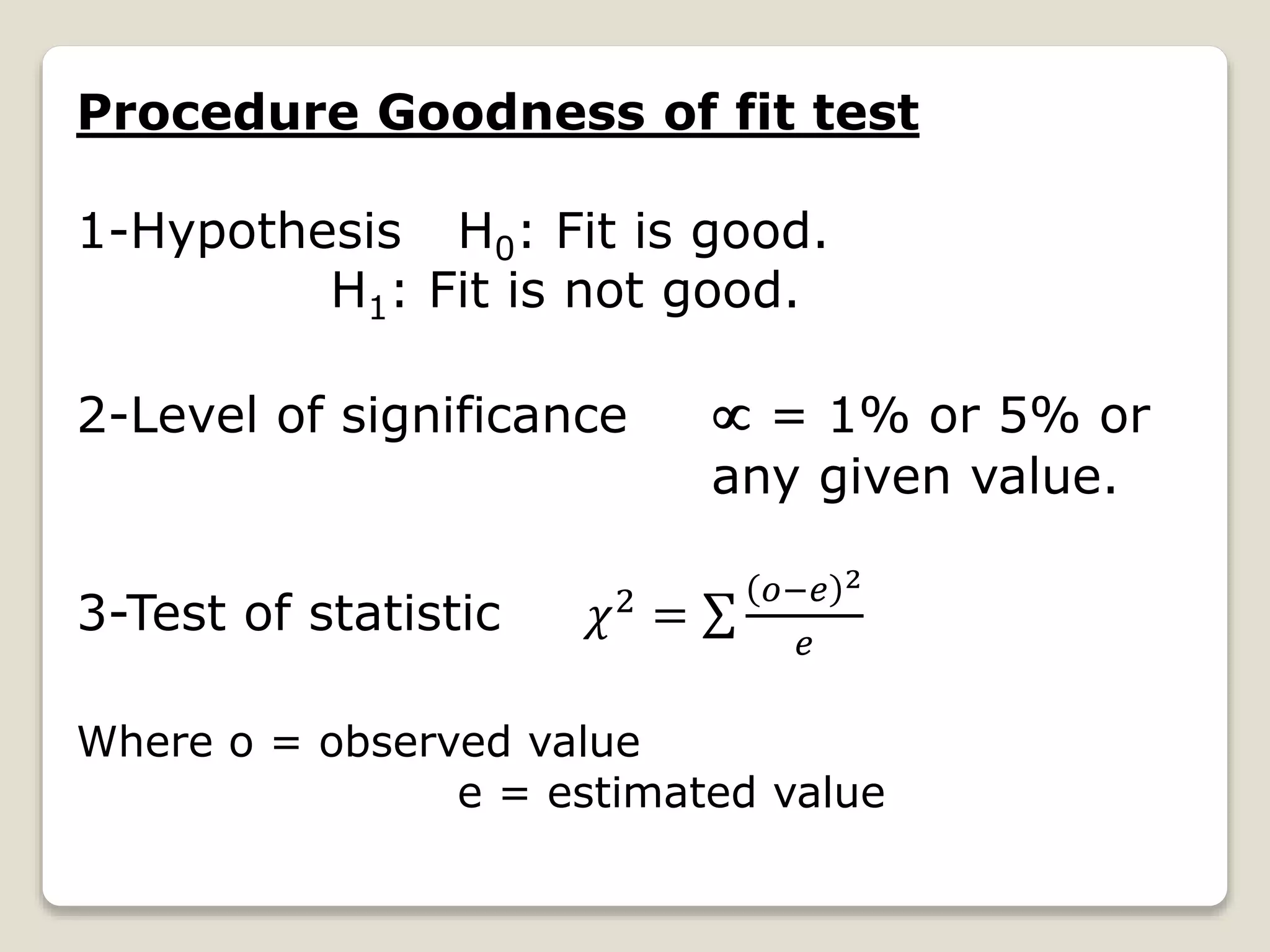
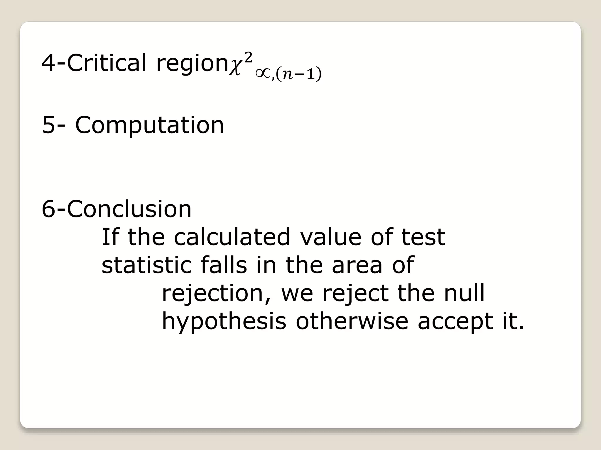
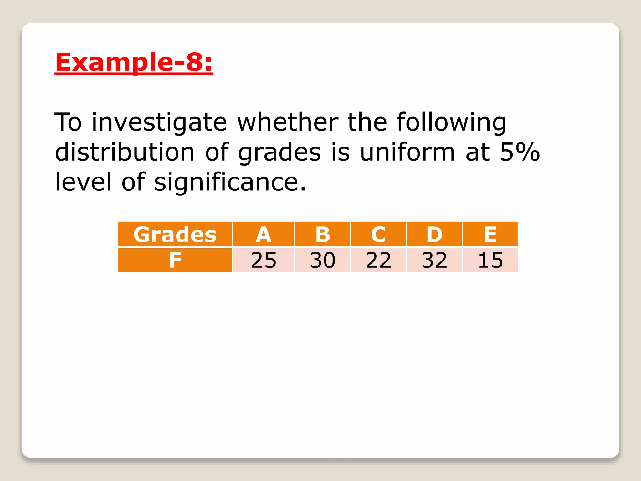
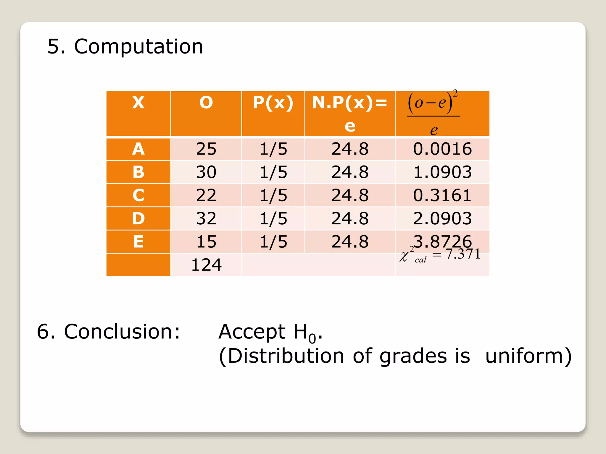
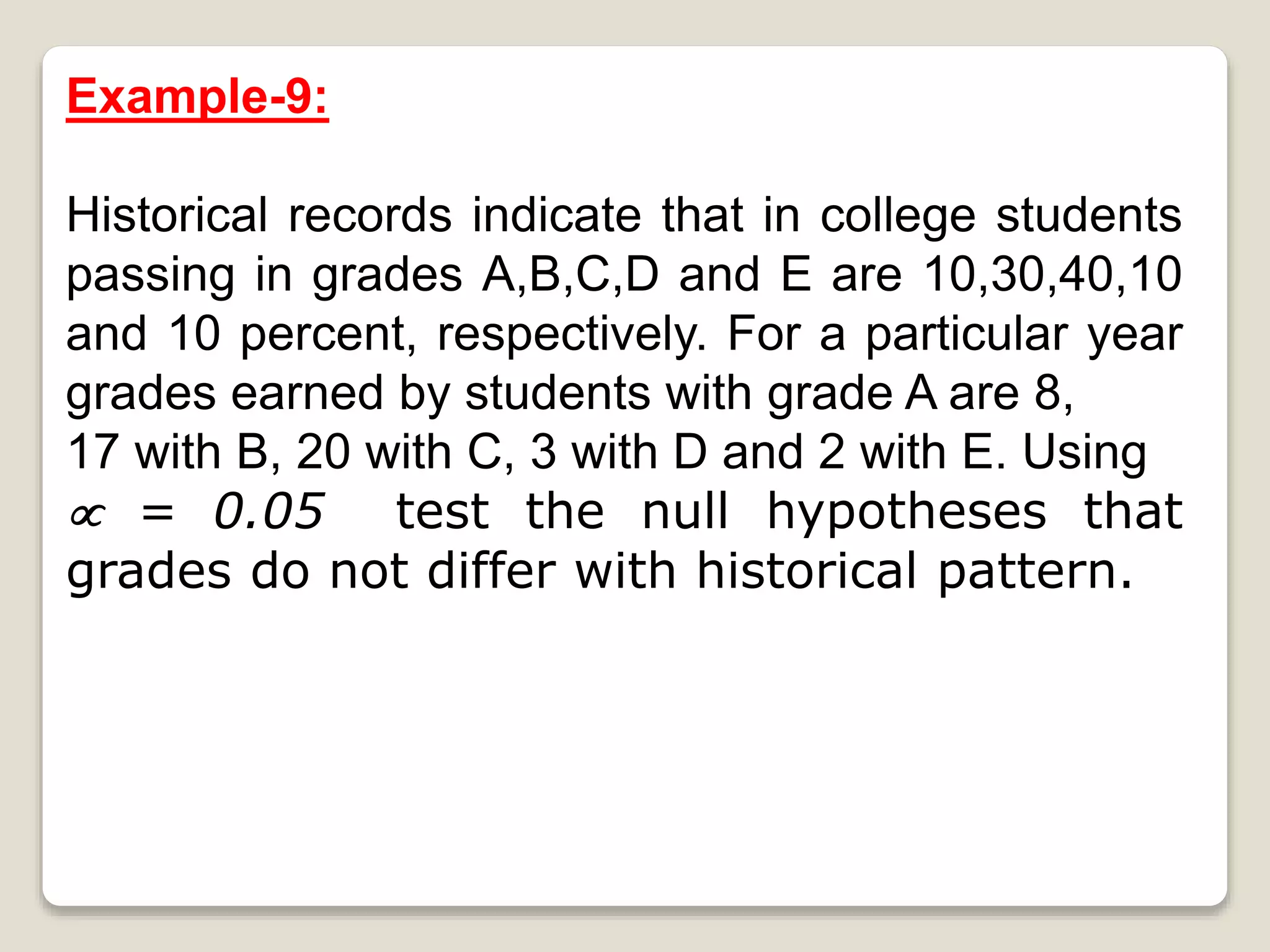
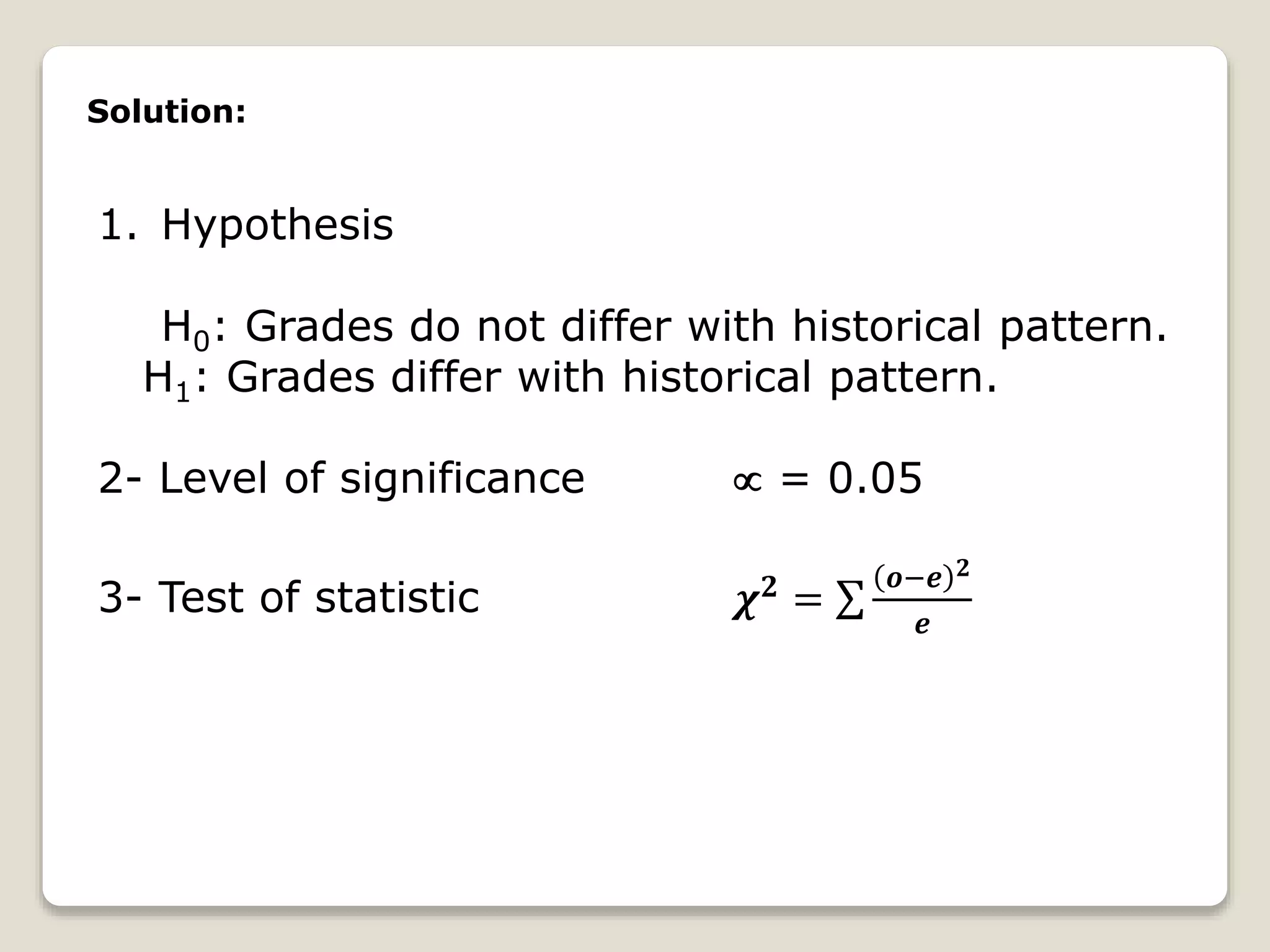
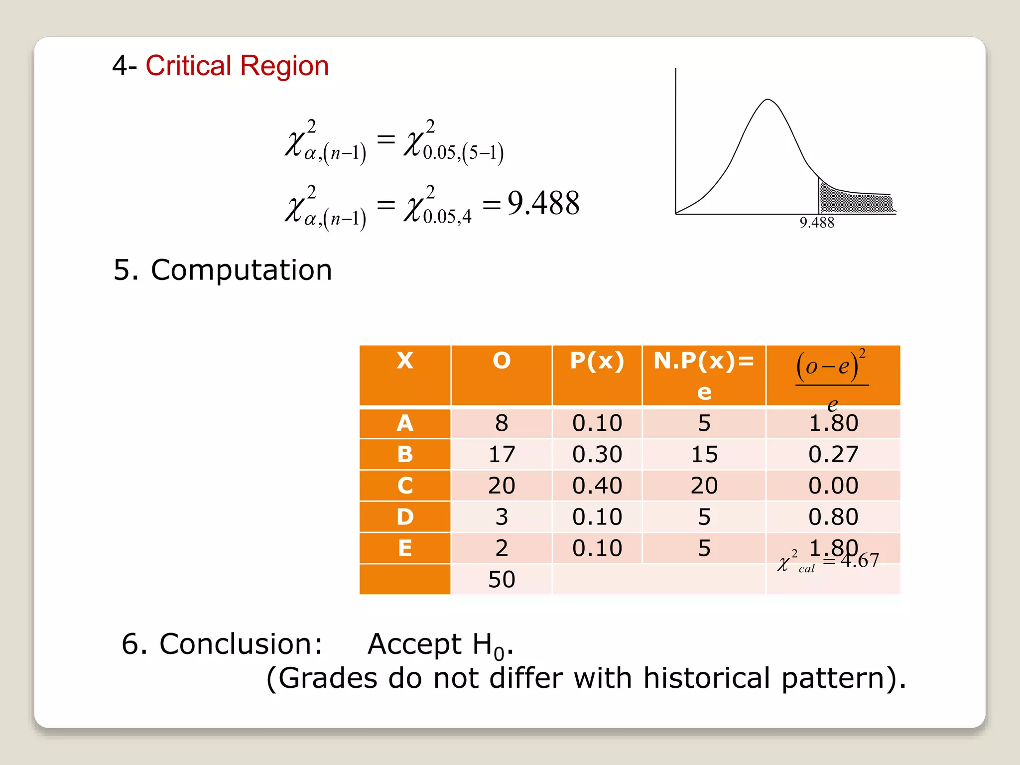
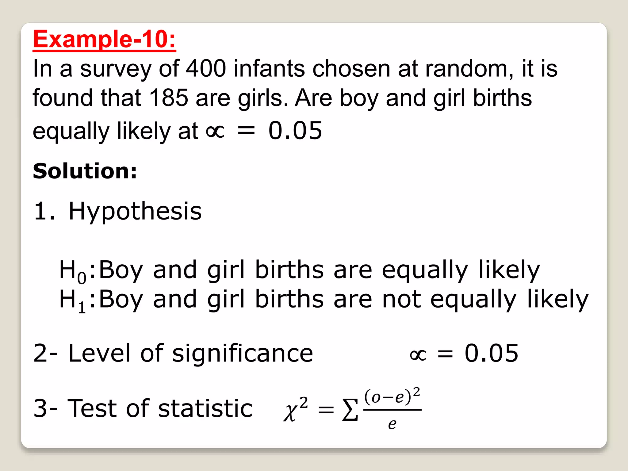
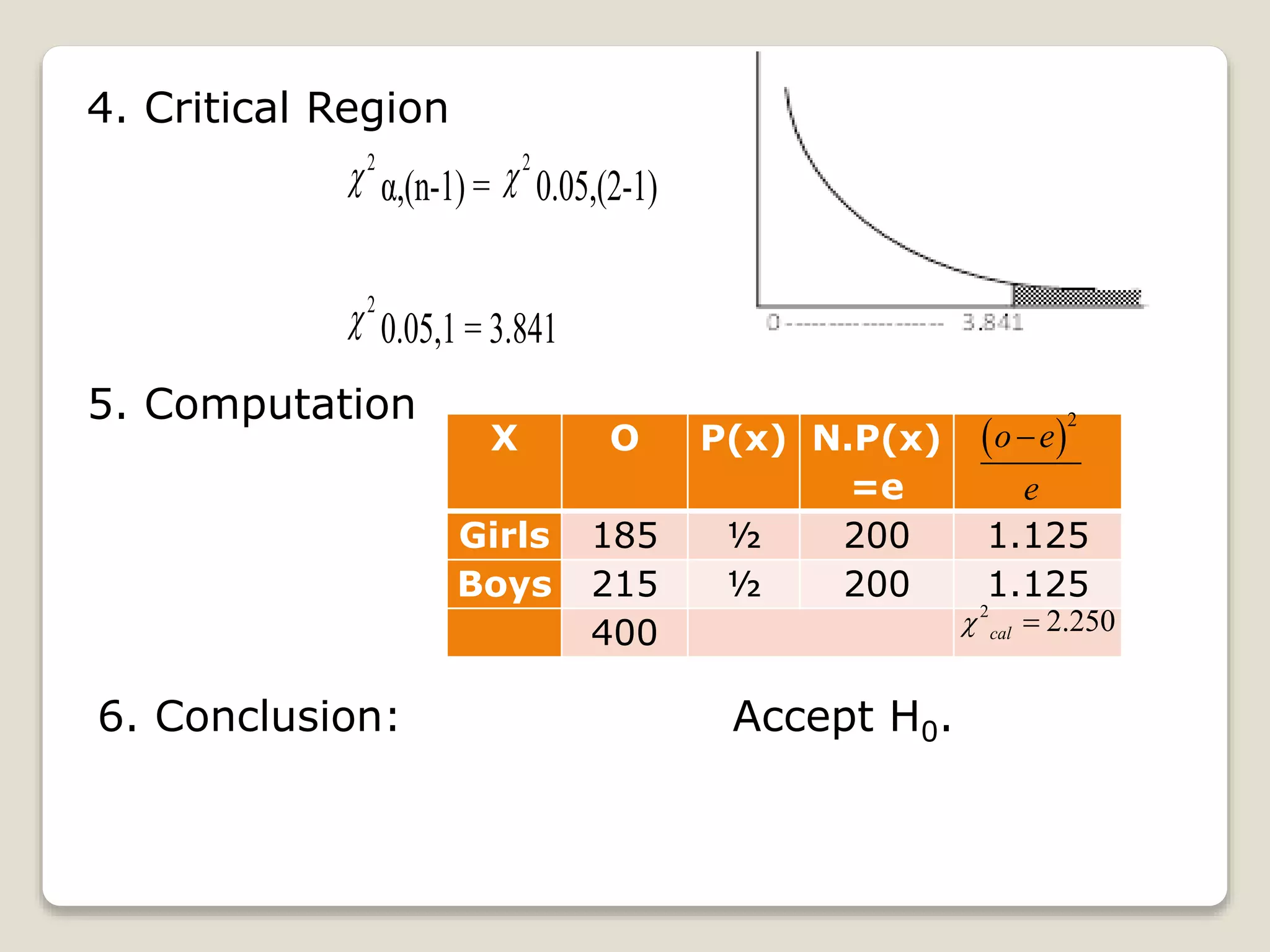
HYPOTHESIS
TESTING
Chi-Square Goodness of Fit Test:
NADEEM UDDIN
ASSOCIATE PROFESSOR
OF STATISTICS
Chi-Square Goodness of Fit Test:
This lesson explains how to conduct a chi-
square goodness of fit test. The test is
applied when you have one categorical
variable from a single population. It is
used to determine whether sample data
are consistent with a hypothesized
distribution.
Procedure Goodness of fit test
1-Hypothesis H0: Fit is good.
H1: Fit is not good.
2-Level of significance  = 1% or 5% or
any given value.
3-Test of statistic 𝜒2 =
𝑜−𝑒 2
𝑒
Where o = observed value
e = estimated value
4-Critical region𝜒2
, 𝑛−1
5- Computation
6-Conclusion
If the calculated value of test
statistic falls in the area of
rejection, we reject the null
hypothesis otherwise accept it.
Example-8:
To investigate whether the following
distribution of grades is uniform at 5%
level of significance.
Grades A B C D E
F 25 30 22 32 15
Solution:
1- Hypothesis H0: Distribution of grades is uniform.
H1:Distribution of grades is not uniform.
2- Level of significance  = 0.05
3- Test of statistic 𝝌 𝟐
=
𝒐−𝒆 𝟐
𝒆
4- Critical region    
 
2 2
, 1 0.05, 5 1
2 2
0.05,4, 1
9.488
n
n


 
 
 


 
9.488
5. Computation
X O P(x) N.P(x)=
e
A 25 1/5 24.8 0.0016
B 30 1/5 24.8 1.0903
C 22 1/5 24.8 0.3161
D 32 1/5 24.8 2.0903
E 15 1/5 24.8 3.8726
124
 
2
o e
e

2
7.371cal 
6. Conclusion: Accept H0.
(Distribution of grades is uniform)
Example-9:
Historical records indicate that in college students
passing in grades A,B,C,D and E are 10,30,40,10
and 10 percent, respectively. For a particular year
grades earned by students with grade A are 8,
17 with B, 20 with C, 3 with D and 2 with E. Using
 = 0.05 test the null hypotheses that
grades do not differ with historical pattern.
Solution:
1. Hypothesis
H0: Grades do not differ with historical pattern.
H1: Grades differ with historical pattern.
2- Level of significance  = 0.05
3- Test of statistic 𝝌 𝟐 =
𝒐−𝒆 𝟐
𝒆
   
 
2 2
, 1 0.05, 5 1
2 2
0.05,4, 1
9.488
n
n


 
 
 


  9.488
4- Critical Region
5. Computation
6. Conclusion: Accept H0.
(Grades do not differ with historical pattern).
X O P(x) N.P(x)=
e
A 8 0.10 5 1.80
B 17 0.30 15 0.27
C 20 0.40 20 0.00
D 3 0.10 5 0.80
E 2 0.10 5 1.80
50
 
2
o e
e

2
4.67cal 
Example-10:
In a survey of 400 infants chosen at random, it is
found that 185 are girls. Are boy and girl births
equally likely at  = 0.05
Solution:
1. Hypothesis
H0:Boy and girl births are equally likely
H1:Boy and girl births are not equally likely
2- Level of significance  = 0.05
3- Test of statistic 𝜒2 =
𝑜−𝑒 2
𝑒
4. Critical Region
2
 α,(n-1) =
2
 0.05,(2-1)
2
 0.05,1 = 3.841
5. Computation
X O P(x) N.P(x)
=e
Girls 185 ½ 200 1.125
Boys 215 ½ 200 1.125
400
 
2
o e
e

2
2.250cal 
6. Conclusion: Accept H0.

Hypothesis testing chi square goodness of fit test

  • 1.
    HYPOTHESIS TESTING Chi-Square Goodness ofFit Test: NADEEM UDDIN ASSOCIATE PROFESSOR OF STATISTICS
  • 2.
    Chi-Square Goodness ofFit Test: This lesson explains how to conduct a chi- square goodness of fit test. The test is applied when you have one categorical variable from a single population. It is used to determine whether sample data are consistent with a hypothesized distribution.
  • 3.
    Procedure Goodness offit test 1-Hypothesis H0: Fit is good. H1: Fit is not good. 2-Level of significance  = 1% or 5% or any given value. 3-Test of statistic 𝜒2 = 𝑜−𝑒 2 𝑒 Where o = observed value e = estimated value
  • 4.
    4-Critical region𝜒2 , 𝑛−1 5-Computation 6-Conclusion If the calculated value of test statistic falls in the area of rejection, we reject the null hypothesis otherwise accept it.
  • 5.
    Example-8: To investigate whetherthe following distribution of grades is uniform at 5% level of significance. Grades A B C D E F 25 30 22 32 15
  • 6.
    Solution: 1- Hypothesis H0:Distribution of grades is uniform. H1:Distribution of grades is not uniform. 2- Level of significance  = 0.05 3- Test of statistic 𝝌 𝟐 = 𝒐−𝒆 𝟐 𝒆 4- Critical region       2 2 , 1 0.05, 5 1 2 2 0.05,4, 1 9.488 n n             9.488
  • 7.
    5. Computation X OP(x) N.P(x)= e A 25 1/5 24.8 0.0016 B 30 1/5 24.8 1.0903 C 22 1/5 24.8 0.3161 D 32 1/5 24.8 2.0903 E 15 1/5 24.8 3.8726 124   2 o e e  2 7.371cal  6. Conclusion: Accept H0. (Distribution of grades is uniform)
  • 8.
    Example-9: Historical records indicatethat in college students passing in grades A,B,C,D and E are 10,30,40,10 and 10 percent, respectively. For a particular year grades earned by students with grade A are 8, 17 with B, 20 with C, 3 with D and 2 with E. Using  = 0.05 test the null hypotheses that grades do not differ with historical pattern.
  • 9.
    Solution: 1. Hypothesis H0: Gradesdo not differ with historical pattern. H1: Grades differ with historical pattern. 2- Level of significance  = 0.05 3- Test of statistic 𝝌 𝟐 = 𝒐−𝒆 𝟐 𝒆
  • 10.
         2 2 , 1 0.05, 5 1 2 2 0.05,4, 1 9.488 n n             9.488 4- Critical Region 5. Computation 6. Conclusion: Accept H0. (Grades do not differ with historical pattern). X O P(x) N.P(x)= e A 8 0.10 5 1.80 B 17 0.30 15 0.27 C 20 0.40 20 0.00 D 3 0.10 5 0.80 E 2 0.10 5 1.80 50   2 o e e  2 4.67cal 
  • 11.
    Example-10: In a surveyof 400 infants chosen at random, it is found that 185 are girls. Are boy and girl births equally likely at  = 0.05 Solution: 1. Hypothesis H0:Boy and girl births are equally likely H1:Boy and girl births are not equally likely 2- Level of significance  = 0.05 3- Test of statistic 𝜒2 = 𝑜−𝑒 2 𝑒
  • 12.
    4. Critical Region 2 α,(n-1) = 2  0.05,(2-1) 2  0.05,1 = 3.841 5. Computation X O P(x) N.P(x) =e Girls 185 ½ 200 1.125 Boys 215 ½ 200 1.125 400   2 o e e  2 2.250cal  6. Conclusion: Accept H0.