• The test(pronounced as chi-square test) is an important and popular
test of hypothesis which fall is categorized in non-parametric test.
• This test was first introduced by Karl Pearson in the year 1900.
•The most obviousdifference between the
chi‑square tests and the other hypothesis
tests we have considered (T test) is the
nature of the data.
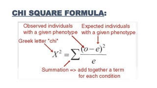
•For chi‑square, the data are frequencies
rather than numerical scores.
5.
•For testing significanceof patterns in qualitative
data.
•Test statistic is based on counts that represent the
number of items that fall in each category
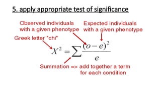
•Test statistics measures the agreement between
actual counts(observed) and expected counts
assuming the null hypothesis
Chi-squared Tests
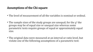
Assumptions of theChi-square
• The level of measurement of all the variables is nominal or ordinal.
• The sample sizes of the study groups are unequal; for the χ2
the
groups may be of equal size or unequal size whereas some
parametric tests require groups of equal or approximately equal
size.
• The original data were measured at an interval or ratio level, but
violate one of the following assumptions of a parametric test:
9.
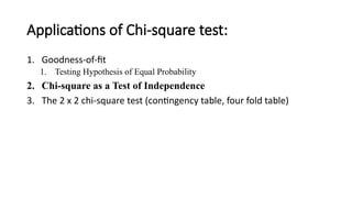
Applications of Chi-squaretest:
1. Goodness-of-fit
1. Testing Hypothesis of Equal Probability
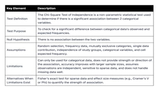
2. Chi-square as a Test of Independence
3. The 2 x 2 chi-square test (contingency table, four fold table)
10.
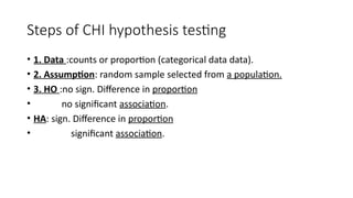
Steps of CHIhypothesis testing
• 1. Data :counts or proportion (categorical data data).
• 2. Assumption: random sample selected from a population.
• 3. HO :no sign. Difference in proportion
• no significant association.
• HA: sign. Difference in proportion
• significant association.
11.
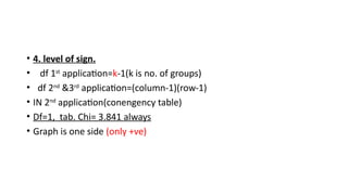
• 4. levelof sign.
• df 1st
application=k-1(k is no. of groups)
• df 2nd
&3rd
application=(column-1)(row-1)
• IN 2nd
application(conengency table)
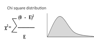
• Df=1, tab. Chi= 3.841 always
• Graph is one side (only +ve)
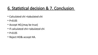
6. Statistical decision& 7. Conclusion
• Calculated chi <tabulated chi
• P>0.05
• Accept HO,(may be true)
• If calculated chi> tabulated chi
• P<0.05
• Reject HO& accept HA.
15.
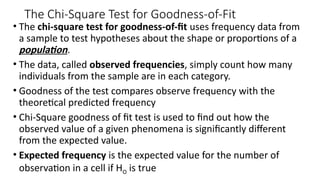
The Chi-Square Testfor Goodness-of-Fit
• The chi-square test for goodness-of-fit uses frequency data from
a sample to test hypotheses about the shape or proportions of a
population.
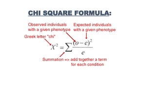
• The data, called observed frequencies, simply count how many
individuals from the sample are in each category.
• Goodness of the test compares observe frequency with the
theoretical predicted frequency
• Chi-Square goodness of fit test is used to find out how the
observed value of a given phenomena is significantly different
from the expected value.
• Expected frequency is the expected value for the number of
observation in a cell if HO is true
16.
• In ChiSquaregoodness of fit test, the term goodness of fit is used in
order to compare the observed sample distribution with the expected
probability distribution.
• Chi-Square goodness of fit test determines how well theoretical
distribution (such as normal, binomial, or Poisson) fits the empirical
distribution. In Chi-Square goodness of fit test, sample data is divided
into intervals. Then the numbers of points that fall into the interval
are compared, with the expected numbers of points in each interval.
17.
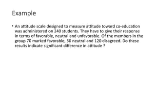
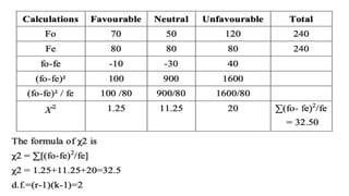
Example
• An attitudescale designed to measure attitude toward co-education
was administered on 240 students. They have to give their response
in terms of favorable, neutral and unfavorable. Of the members in the
group 70 marked favorable, 50 neutral and 120 disagreed. Do these
results indicate significant difference in attitude ?
19.
1. Data
•Represents 240students.
•the group marked :- 70 favorable, 50 neutral and 120
disagreed.
19
3. Hypothesis
• Nullhypothesis: there is no significant difference in
proportion of measure attitude toward co-education.
• Alternative hypothesis: there is significant difference in
proportion of measure attitude toward co-education.
21
22.
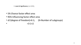
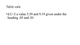
4. Level ofsignificance; (α =0.05);
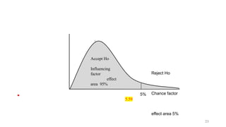
• 5% Chance factor effect area
• 95% Influencing factor effect area
• d.f.(degree of freedom)=K-1; (K=Number of subgroups)
• =3-1=2
22
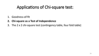
Applications of Chi-squaretest:
1. Goodness-of-fit
2. Chi-square as a Test of Independence
3. The 2 x 2 chi-square test (contingency table, four fold table)
34
35.
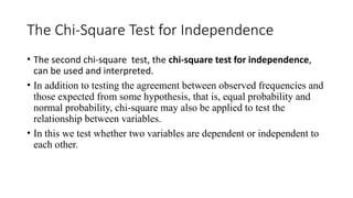
The Chi-Square Testfor Independence
• The second chi-square test, the chi-square test for independence,
can be used and interpreted.
• In addition to testing the agreement between observed frequencies and
those expected from some hypothesis, that is, equal probability and
normal probability, chi-square may also be applied to test the
relationship between variables.
• In this we test whether two variables are dependent or independent to
each other.
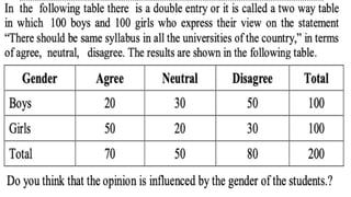
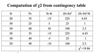
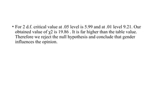
• For 2d.f. critical value at .05 level is 5.99 and at .01 level 9.21. Our
obtained value of χ2 is 19.86 . It is far higher than the table value.
Therefore we reject the null hypothesis and conclude that gender
influences the opinion.
42.
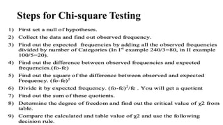
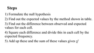
Steps
1) Formulate thenull hypothesis
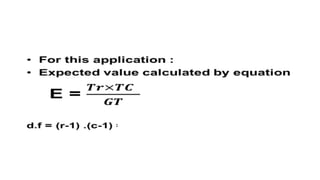
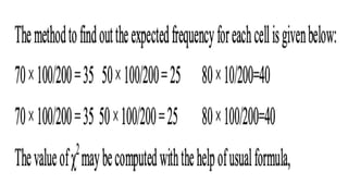
2) Find out the expected values by the method shown in table.
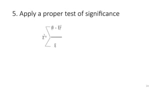
3) Find out the difference between observed and expected
values for each cell.
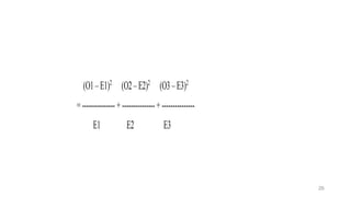
4) Square each difference and divide this in each cell by the
expected frequency.
5) Add up these and the sum of these values gives χ2
43.
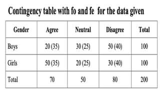
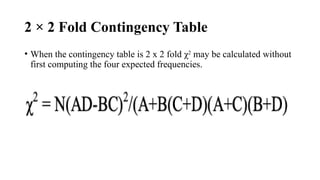
2 × 2Fold Contingency Table
• When the contingency table is 2 x 2 fold χ2
may be calculated without
first computing the four expected frequencies.