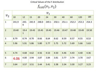
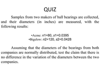
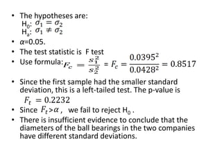
Here are the steps to solve this problem: 1) State the null and alternative hypotheses: H0: σ1^2 = σ2^2 (the variances are equal) Ha: σ1^2 ≠ σ2^2 (the variances are unequal) 2) Specify the significance level: α = 0.05 3) Calculate the F-statistic: F = (0.0428/120) / (0.0395/80) = 1.0833 4) Find the p-value: This is a left-tailed test since s1 < s2. From the F-distribution table with degrees of freedom v1 = 80-1

1. F- Distribution

2. F- Distribution
Theoretically, we might define the F distribution to
be the ratio of two independent chi-square distributions,
each divided by their degrees of freedom. Hence, if f is a
value of the random variable F, we have:
F= = =
Where X12 is a value of a chi-square distribution with v1= n1-1 degrees
of freedom and X22 is a value of a chi-square distribution with v2= n2-1
degrees of freedom. We say that f is a value of the F- distribution with
v1 and v2 degrees of freedom.

3. To obtain an f value, first select a random sample of size n1 from a normal
Population having a variance and compute .
An independent sample of size n, is then selected from a second
normal population with variance and is computed.
The ratio of the two quantities
and is the denominator is called the F- distribution, with v1 and
v2 degrees of freedom.

4. • The number of degrees of freedom associated
with the sample variance in the numerator is
always stated first, followed by the number of
degrees of freedom associated with the
sample variance in the denominator. Thus the
curve of the F distribution depends not only
on the two parameters v1 and v2 but also on
the order in which we state them. Once
these two values are given, we can identify
the curve.

5. 6 and 24 degrees of freedom
6 and 10 degrees of freedom
TYPICAL
F DISTRIBUTION

6. • Let be the f value above which we find an
area equal to . This is illustrated by the
shaded region.
• Example: The f value with 6 and 10 degrees of
freedom, leaving an area of 0.05 to the right,
is = 3.22. By means of the following
theorem, Table A.7 can be used to find values
of and .

7. Tabulated Values of the F- Distribution
0 f

8. • Writing for with v1 and v2 degrees
of freedom. THEN,
Thus the f value with 6 and 10 degrees of freedom, leaving an area of 0.95
to the right, is
=

9. Critical Values of the F distribution
10 12 15 20 24 30 40 60 120
1 241.9 243. 245.9 248.0 249.1 250.1 251.1 252.2 253.3 254.3
9
2 19.40 19.4 19.43 19.45 19.45 19.46 19.47 19.48 19.49 19.50
1
3 8.79 8.74 8.70 8.66 8.64 8.62 8.59 8.57 8.55 8.53
4 5.96 5.91 5.86 5.80 5.77 5.75 5.72 5.69 5.66 5.63
5 4.74 4.68 4.62 4.56 4.53 4.50 4.46 4.43 4.40 4.36
6 4.00 3.94 3.87 3.84 3.81 3.77 3.74 3.70 3.67
4.06
7 3.64 3.57 3.51 3.44 3.41 3.38 3.34 3.30 3.27 3.23

10. • The F distribution is applied primarily in the
analysis of variance where we wish to test the
equality of several means simultaneously. We
shall use the F distribution to make inferences
concerning the variance of two normal
populations.

11. TEST ABOUT TWO VARIANCES OR
STANDARD DEVIATION

12. FORMULA:
Where :
is the greater variance
is the smaller variance

13. • Example 9.1.31.
A group of Mass Communication students
study telephone calls at the registrar’s office.
The students monitor the time of the
incoming and outgoing calls for one day. They
that 17 incoming calls last an average of 4.13
minutes with a variance of 1.36 test the
hypothesis that the variances of the samples
are equal. Use the 0.05 level of significance.

14. • Solution: We follow the steps in hypothesis
testing.
a. H0 : The variances of the samples are equal.
b. Ha : The variances of the samples are not
equal

15. c. Set
d. Tabular value of F. Use F-test (test about two
variances or standard deviations)
v = (17-1, 12-1)
e. Computed value of F

16. f. Conclusion: Since , accept H0. Hence,
the variances of the samples are equal.

17. Here’s the Solution:
a. H0 : The two samples come from the
population with equal variances.
b. Ha : The two samples come from the
population with smaller variances

18. SEATWORK:
From sample of 25 observations, the
estimate of the standards, the estimate of the
variance of the population was found to 15.0
From another sample of 14 observations, the
estimate variance was found to be 9.7 Can we
accept the hypothesis that the two samples
come from populations with equal variance,
or must we conclude that the variance of the
second population is smaller? Use the 0.01
level of significance.

20. c. Set
d. Tabular value of F. Use F-test.
v = (25-1, 14-1)
e. Computed value of F
f. Conclusion: Since , accept H0. Hence,
the two samples come from the population
with equal variances.

21. PROCEED TO THE FAVORITE PART

22. QUIZ
Samples from two makers of ball bearings are collected,
and their diameters (in inches) are measured, with the
following results:
•Acme: n1=80, s1=0.0395
•Bigelow: n2=120, s2=0.0428
Assuming that the diameters of the bearings from both
companies are normally distributed, test the claim that there is
no difference in the variation of the diameters between the two
companies.

23. LET’s CHECK!

24. • The hypotheses are:
H0:
Ha :
• α=0.05.
• The test statistic is F test
• Use formula: =
• Since the first sample had the smaller standard
deviation, this is a left-tailed test. The p-value is
• Since > , we fail to reject H0 .
• There is insufficient evidence to conclude that the
diameters of the ball bearings in the two companies
have different standard deviations.