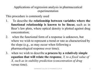
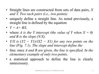
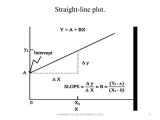
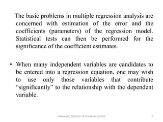
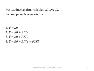
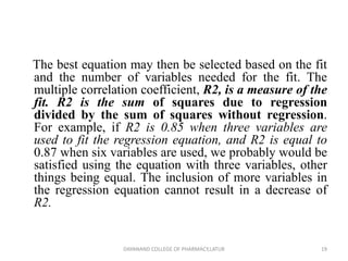
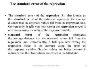
Regression analysis is a statistical technique for investigating relationships between variables. Simple linear regression defines a relationship between two variables (X and Y) using a best-fit straight line. Multiple regression extends this to model relationships between a dependent variable Y and multiple independent variables (X1, X2, etc.). Regression coefficients are estimated to define the regression equation, and R-squared and the standard error can be used to assess the goodness of fit of the regression model to the data. Regression analysis has applications in pharmaceutical experimentation such as analyzing standard curves for drug analysis.

1. Regression
Ms. Shraddha S. Tiwari
Assistant Professor
Dayanand Education Society's
Dayanand College of Pharmacy,
SRTMUN.
1
DAYANAND COLLEGE OF PHARMACY,LATUR

2. Regression
Simple linear regression analysis is a statistical
technique that defines the functional relationship
between two variables, X and Y, by the “best-
fitting” straight line.
A straight line is described by the equation,
Y = A + BX, where Y is the dependent variable
(ordinate), X is the independent variable
(abscissa), and A and B are the Y intercept and
slope of the line, respectively.
2
DAYANAND COLLEGE OF PHARMACY,LATUR

3. Applications of regression analysis in pharmaceutical
experimentation
This procedure is commonly used
1. To describe the relationship between variables where the
functional relationship is known to be linear, such as in
Beer’s law plots, where optical density is plotted against drug
concentration;
2. when the functional form of a response is unknown, but
where we wish to represent a trend or rate as characterized by
the slope (e.g., as may occur when following a
pharmacological response over time);
3. when we wish to describe a process by a relatively simple
equation that will relate the response, Y, to a fixed value of
X, such as in stability prediction (concentration of drug
versus time).
3
DAYANAND COLLEGE OF PHARMACY,LATUR

4. • Straight lines are constructed from sets of data pairs, X
and Y. Two such pairs (i.e., two points)
• uniquely define a straight line. As noted previously, a
straight line is defined by the equation
• Y = A+ BX,
• where A is the Y intercept (the value of Y when X = 0)
and B is the slope (Y/X).
• Y/X is (Y2 − Y1)/(X2 − X1) for any two points on the
line (Fig. 7.1). The slope and intercept define the
• line; once A and B are given, the line is specified. In the
elementary example of only two points,
• a statistical approach to define the line is clearly
unnecessary.
4
DAYANAND COLLEGE OF PHARMACY,LATUR

5. Straight-line plot.
5
DAYANAND COLLEGE OF PHARMACY,LATUR

6. • In this example, the equation of the line Y = A
+ BX is Y = 0 + 1(X), or Y = X. Since there is
no error in this experiment, the line passes
exactly through the four X, Y points.
• calculus, the slope and intercept of the least
squares line can be calculated from the sample
data as follows:
• Slope = b = (X − X)(y − y) / ∑(X − X)2
• Intercept = a = y − bX
• Remember that the slope and intercept
uniquely define the line. 6
DAYANAND COLLEGE OF PHARMACY,LATUR

7. • There is a shortcut computing formula for the
slope, similar to that described previously
for the standard deviation
• b = (N∑Xy) − (∑X)( ∑y)
N ∑ X2 − (∑ X)2
7
DAYANAND COLLEGE OF PHARMACY,LATUR

8. Raw Data to Calculate the Least
Squares Line
Drug potency, X Assay, y Xy
60 60 3600
80 80 6400
100 100 10,000
120 120 14,400
∑ X= 360 ∑ y = 360 ∑ Xy = 34,400
∑ X 2 = 34,400
8
DAYANAND COLLEGE OF PHARMACY,LATUR

9. • For the example shown in Figure 7.2(A), the line that exactly
passes through the four data points has a slope of 1 and an
intercept of 0. The line, Y = X, is clearly the best line for these
data, an exact fit. The least squares line, in this case, is exactly
the same line, Y = X. The calculation of the intercept and slope
using the least squares formulas, Eqs. (7.3) and (7.4), is
illustrated below.
• Table 7.1 shows the raw data used to construct the line in
Figure 7.2(A).
• According to Eq. (7.4) (N = 4, ∑X2 = 34,400, ∑ Xy = 34,400,
• ∑ X = ∑ y = 360),
b = (4)(3600 + 6400 + 10,000 + 14,000) − (360)(360)
4(34,400) − (360)2
= 1
9
DAYANAND COLLEGE OF PHARMACY,LATUR

10. • a is computed fromEq. (7.3); a = y − bX(y = X = 90,
b = 1). a = 90 − 1(90) = 0. This represents a situation
where the assay results exactly equal the known drug
potency (i.e., there is no error).
• A perfect assay (no error) has a slope of 1 and an
intercept of 0, as shown above. The actual data
exhibit a slope close to 1, but the intercept appears to
be too far from 0 to be attributed to random error.
10
DAYANAND COLLEGE OF PHARMACY,LATUR

11. Raw Data used to Calculate the Least Squares Line
Drug potency, X Assay, y Xy
60 63 3780
80 75 6000
100 99 9900
120 116 13920
∑ X= 360 ∑ y = 353 ∑ Xy = 33,600
∑ x2 = 34400 ∑ y 2 = 32851
11
DAYANAND COLLEGE OF PHARMACY,LATUR

12. • b = (4)(33,600) − (360)(353)
4(34,400) − (360)2 = 0.915.
• a = 353 − 0.915(90) = 5.9
4.
Assay result = 5.9 + 0.915 (potency).
• Potency = X = y − 5.9
0.915
• Potency = 90 − 5.9
0.915
= 91.9.
12
DAYANAND COLLEGE OF PHARMACY,LATUR

13. ANALYSIS OF STANDARD CURVES IN DRUG ANALYSIS:
APPLICATION OF LINEAR REGRESSION
The assay data discussed previously can be considered
as an example of the construction of a standard curve
in drug analysis. Known amounts of drug are
subjected to an assay procedure, and a plot of
percentage recovered (or amount recovered) versus
amount added is constructed. Theoretically, the
relationship is usually a straight line. A knowledge of
the line parameters A and B can be used to predict the
amount of drug in an unknown sample based on the
assay results. In most practical situations, A and B are
unknown. The least squares estimates a and b of these
parameters are used to compute drug potency (X)
based on the assay response (y). For example, the
least squares line for the data in Figure 7.2(B) and
Table 7.2 is 13
DAYANAND COLLEGE OF PHARMACY,LATUR

14. Multiple Regression
• Multiple regression is an extension of linear
regression, in which we wish to relate a
response, Y (dependent variable), to more than
one independent variable, Xi.
• Linear regression: Y = A+ BY
• Multiple regression: Y = B0 + B1X1 + B2X2 +
...
• The independent variables, X1, X2, and so on,
14
DAYANAND COLLEGE OF PHARMACY,LATUR

15. • Y = B0 + B1X1 + B2X2 + B3X3,
• where Y is the some measure of dissolution, Xi is ith
independent variable, and Bi the regression coefficient for
the ith independent variable.
• Here, X1, X2, and X3 refer to the level of disintegrant,
lubricant, and drug. B1, B2, and B3 are the coefficients
relating the Xi to the response. These coefficients
correspond to the slope (B) in linear regression. B0 is the
intercept. This equation cannot be simply depicted,
graphically, as in the linear regression case. With two
independent variables (X1 and X2), the response surface
• is a plane (Fig. III.1). With more than two independent
variables, it is not possible to graph the response in two
dimensions.
15
DAYANAND COLLEGE OF PHARMACY,LATUR

16. Representation of the multiple regression
equation response, Y = B0 + B1×1 + B2X 2, as a plane.
16
DAYANAND COLLEGE OF PHARMACY,LATUR

17. The basic problems in multiple regression analysis are
concerned with estimation of the error and the
coefficients (parameters) of the regression model.
Statistical tests can then be performed for the
significance of the coefficient estimates.
• When many independent variables are candidates to
be entered into a regression equation, one may wish
to use only those variables that contribute
“significantly” to the relationship with the dependent
variable.
17
DAYANAND COLLEGE OF PHARMACY,LATUR

18. For two independent variables, X1 and X2,
the four possible regressions are
1. Y = B0
2. Y = B0 + B1X1
3. Y = B0 + B2X2
4. Y = B0 + B1X1 + B2X2
18
DAYANAND COLLEGE OF PHARMACY,LATUR

19. The best equation may then be selected based on the fit
and the number of variables needed for the fit. The
multiple correlation coefficient, R2, is a measure of the
fit. R2 is the sum of squares due to regression
divided by the sum of squares without regression.
For example, if R2 is 0.85 when three variables are
used to fit the regression equation, and R2 is equal to
0.87 when six variables are used, we probably would be
satisfied using the equation with three variables, other
things being equal. The inclusion of more variables in
the regression equation cannot result in a decrease of
R2.
19
DAYANAND COLLEGE OF PHARMACY,LATUR

20. The standard error of the regression
• The standard error of the regression (S), also known as
the standard error of the estimate, represents the average
distance that the observed values fall from the regression line.
Conveniently, it tells you how wrong the regression model is
on average using the units of the response variable.
• standard error of the regression represents
the average distance that the observed values fall from the
regression line. Conveniently, it tells you how wrong the
regression model is on average using the units of
the response variable. Smaller values are better because it
indicates that the observations are closer to the fitted line.
20
DAYANAND COLLEGE OF PHARMACY,LATUR

21. • Unlike R-squared value, you can use the
standard error of the regression to assess the
precision of the predictions. Approximately
95% of the observations should fall within
plus/minus 2*standard error of the regression
from the regression line, which is also a quick
approximation of a 95% prediction interval. If
want to use a regression model to make
predictions, assessing the standard error of the
regression might be more important than
assessing R-squared.
21
DAYANAND COLLEGE OF PHARMACY,LATUR

22. R-squared
• R-squared is the percentage of the response variable
variation that is explained by a linear model. It is always
between 0 and 100%. R-squared is a statistical measure of
how close the data are to the fitted regression line. It is also
known as the coefficient of determination, or the coefficient
of multiple determination for multiple regression.
• In general, the higher the R-squared, the better the model
fits your data. However, there are important conditions for
this guideline that I discuss elsewhere. Before you can trust
the statistical measures for goodness-of-fit, like R-squared,
you should check the residual plots for unwanted patterns
that indicate biased results.
22
DAYANAND COLLEGE OF PHARMACY,LATUR

23. Thank you …
23
DAYANAND COLLEGE OF PHARMACY,LATUR