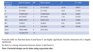
The document covers the design and analysis of experiments with a focus on factorial design, detailing its historical development, advantages, and disadvantages. It describes key designs in experiments, including completely randomized, randomized complete block, and factorial designs, along with statistical methods such as ANOVA for analyzing experimental data. Additionally, practical examples illustrate how factorial experiments assess the effects of multiple factors simultaneously, highlighting efficiency and the complexity of statistical analysis.

1. BIOSTATISTICS AND RESEARCH METHODOLOGY
Unit-5: design and analysis of experiments (Factorial design)
PRESENTED BY
Gokara Madhuri
B. Pharmacy IV Year
UNDER THE GUIDANCE OF
Gangu Sreelatha M.Pharm., (Ph.D)
Assistant Professor
CMR College of Pharmacy, Hyderabad.
email: sreelatha1801@gmail.com

2. • DOE is invented by Sir Ronald Fisher in 1920’s and 1930’s.
• The brief history of design of experiments is summarized in the following 4 eras:
1. The agricultural origin,1918 to 1940 ( R. A .Fisher Frank Yatis ).
• Profound impact on agricultural sciences.
• Development of factorial designs and ANOVA.
2. The first industrial era 1951 to late 1970’s ( Box and Wilson).
• Applications in the chemical and process industries.
3. The second industrial era late 1970’s to 1990 (W. Edward Beming).
• Quality improvement initiatives in many companies.
• Total quality management(TQM) and continuous quality improvement(CQI) were important ideas
and became management goals.
4. The modern era beginning from 1990, when economic competitiveness and globalization is driving
all sectors of economy to be more competitive.
DESIGN OF EXPERIMENTS (DOE)

3. • The following designs of experiments will be usually followed:
1. Completely randomised design(CRD)
2. Randomised complete block design(RCBD)
3. Latin square design(LSD)
4. Factorial design or experiment
5. Confounding
6. Split and strip plot design
FACTORIAL DESIGN:
• When a several factors are investigated simultaneously in a single experiment such experiments are
known as factorial experiments. Though it is not an experimental design, indeed any of the designs
may be used for factorial experiments.
For example, the yield of a product depends on the particular type of synthetic substance used and
also on the type of chemical used.
• If there are ‘p’ different varieties or types then we shall say that there are p levels of the factor variety
or type.
• Similarly, the second factor chemical may have q levels i.e there may be q different chemicals or q
different concentrations of the same chemical.

4. • These factorial design will now be called as pxq experiment.
• In an example the two factors may be 2 different chemicals i.e acetonitrile and methanol and at p and
q different concentrations respectively. This will also give a pxq experiment. We shall consider only
the simplest cases, of ‘n’ factors such as two or three levels are known as 2n ,3n experiments were ‘n’
is any positive integer ≥ 2 .
• If two factors are considered simultaneously the experiment is called two factor factorial experiment.
• If these factors are studied simultaneously as done in the case of latin square were we block two
factors and studied the effect of treatment only, the experiment is called as three factor factorial
experiment.
• The total no of treatments in a factorial experiment is the product of the levels in each factor, in two
square factorial example, the no. of treatments is 2x2=4 and in the 23 factorial the no. of treatments
is 2x2x2=8. The no. of treatments increases rapidly with an increase in the no. of factors or an
increase in the levels in each factor.
• For a factorial experiment involving 5 varieties or types the total no. of treatments would be
5x4x3=60.

5. ADVANTAGES OF FACTORIAL DESIGN
There are many advantages of the factorial experiments:
1. Factorial experiments are advantageous to study the combined effect of two or more factors
simultaneously and analyze their interrelationships. Such factorial experiments are economic in
nature and provide a lot of relevant information about the phenomenon under study. It also
increases the efficiency of the experiment.
2. It is an advantageous because a wide range of factor combination are used. This will give us an idea
to predict about what will happen when two or more factors are used in combination.
3. The factorial approach will result in considerable saving of the time and the experimental materials.
It is because the time required for the combined experiment is less than that required for the
separate experiments.
4. In single factor experiments, the results may not be satisfactory because of the changes in
environmental conditions. However, in factorial experiments such type of difficulties will not arise
even after several factors are investigated simultaneously.
5. Information may obtained from factorial experiments is more complete than that obtained from a
series of single factor experiments, in the sense that factorial experiments permit the evaluation of
interaction effects.

6. DISADVANTAGES
The disadvantages of the factorial experiments are:
• It is disadvantageous because the execution of the experiment and the statistical analysis becomes more
complex when several treatments combinations or factors are involved simultaneously.
• It is also disadvantageous in cases where may not be interested in certain treatment combinations but
we are forced to include them in the experiment. This will lead to wastage of time and also the
experimental material.
• In factorial experiments, the number of treatment combinations will increase if the factors are
increased. This will also lead to the increase in block size, which in turn will increase the
heterogenicity in the experimental material. Because of this it will lead to the increased experimental
error and will decrease the precision in the experiment. Appropriate block size must be maintained.

7. 22 FACTORIAL EXPERIMENT
• A special set of factorial experiment consist of experiments in which all factors have 2 levels such
experiments are referred to generally as 2n factorials.
• If there are four factors each at two levels the experiment is known as 2x2x2x2 or 24 factorial
experiment. On the other hand if there are 2 factors each with 3 levels the experiment is known as 3x3
or 32 factorial experiment. In general if there are n factors each with p levels then it is known as pn
factorial experiment.
• The calculation of the sum of squares is as follows:
Correction factor (CF) =
𝐺𝑇 2
𝑛
GT = grand total
n = total no of observations
• Total sum of squares = 𝑥2 − 𝐶𝐹
• Replication sum of squares (RSS) =
𝑅1 2
+ 𝑅2 2
+⋯+ 𝑅𝑛 2
𝑛
- CF
Or
1
𝑛
𝑅2 − 𝐶𝐹

8. • Treatment sum of squares (TSS) =
𝑇1 2
+ 𝑇2 2
+⋯+ 𝑇𝑛 2
𝑛
− CF
Or
1
𝑛
𝑇2 − 𝐶𝐹
• Residual sum of square = error sum of squares = total sum of square- replication sum of square - TSS
ANOVA TABLE
Example: An experiment was conducted on 4 rabbits in a randomised block design with a four
replications. Analyse the data and conclude the results.
Source of variation Degree of freedom Sum of squares Mean sum of
squares
Factor
Replications r-1 RSS RSS/r-1 RMS/EMS
Treatments t-1 TSS TSS/t-1 TMS/EMS
Error (r-1) (t-1) ESS ESS/(r-1) (t-1) -
Total rt-1 - - -

9. Solution: Null hypothesis ( H0 ) the data do not differ with respect to blocks and treatments.
BLOCK TREATMENT COMBINATIONS
1 l(23) k(25) p(22) kp(38)
2 p(40) l(26) k(36) kp(38)
3 l(29) k(20) kp(30) p(20)
4 kp(34) k(31) p(24) l(28)
Treatment
combination
1 2 3 4 Treatment
totals
l 23 26 29 28 106
k 25 36 20 31 112
p 22 40 20 24 106
kp 38 38 30 34 140
Block total 108 140 99 17 464

10. • Grand total = 464
• Correction factor =
𝐺𝑇 2
𝑛
=
464 2
16
= 13456
• Total sum of square = 𝑥2 − 𝐶𝐹
𝑥2 = 23 2 + 26 2 +(29)2+ (28)2+(25)2+(36)2+(20)2+(31)2 +(22)2+(40)2
+(20)2+(24)2+(38)2+(38)2+(30)2+(34)2 - 13456
= 660
• Replication sum of squares =
108 2
+ 140 2
+ 99 2
+ 17 2
4
-13456
=
54754
4
− 13456
= 13688.5-13456
= 232.5
• TSS =
106 2
+ 112 2
+ 106 2
+ 140 2
4
- 13456
=
11236+12544+11236+19600
4
- 13456

11. =
54616
4
- 13456
= 13654 -13456
= 198
• Residual sum of square = ESS = TSS –RSS -TSS
= 660 -232.5 -198
= 224.5
Source of variation Degree of Freedom Sum of squares Mean sum of squares Factor(f)
Replication 4-1
=3
RSS = 232.5 232.5/3
= 77.5
RMS/EMS =
77.5
25.5
= 3.03
Treatment 4-1
=3
TSS = 198 = 198/3
= 66
TMS/EMS =
66
25.5
= 2.58
Error (r-1) (t-1)
=3X3
=9
229.5 = 229.5/9
= 25.5
Total rt-1
=4X4-1
=16-1
=15

12. Conclusion: The tabulated f value at 5% significance for three degree of freedom is 3.86. The
calculated f value is less than the tabulated value. Therefore, the values are not significant. The data
with respect to blocks and treatments do not differ significantly. So, the null hypothesis is accepted.

13. 23 FACTORIAL DESIGN
• In this type of design, one independent variable has 2 levels, and the other independent variable has 3
levels as shown in the figure 1
• Example: let us imagine that the researcher wants to find the effectiveness of a diet pill A over a
placebo, a dietary regimen B versus usual diet and an exercise regimen C versus usual exercise, on a
weight loss lasting at least a year in adult men.
• In this situation a factorial design can be more efficient and informative because, it allows the
researchers to study not only all the treatments A B C (factors) but allow the precise interactions AB,
BC, AC and also ABC

14. • We have 3 factors of only 2 levels. The levels may be low or high denoted by ‘-’ and ‘+’ respectively.
• The treatment combination is given as
Note (Yates notation)
• The high level of any factor is denoted by the corresponding letter (for example in the above table 2nd
row A is having high level of factor(+) and is denoted by the corresponding letters (a) whereas B and
C are having low levels so the treatment will be denoted by the absence of the corresponding letter.
A B C TREATMENTS
- - - (1)
+ - - a
- + - b
+ + - ab
- - + c
+ - + ac
- + + bc
+ + + abc

15. • The above table can also be represented in a graphical notation
• Design table for treatment
• 1 A B AB C AC BC ABC TREATM
ENTS
+ - - + - + + - 1
+ + - - - - + + a
+ - + - - + - + b
+ + + + - - - - ab
+ - - + + - - + c
+ + - - + + - - ac
+ - + - + - + - bc
+ + + + + + + + abc

16. • In the above table 1st row, A and B are having negative signs(‘-’) so AB becomes(‘+’) (- x - = +) and
in the 2nd row A is having ‘+’ sign and B is having ‘-’ sign so AB becomes (‘-’) (+ x - = -).
• In 3rd row A is having (‘-’) sign and B is having (‘+’)sign so AB becomes(‘-’) ( - x + = -) and in the 4th
row A and B are having (‘+’) signs so AB becomes(‘+’) (+ x + = +)
• In ABC it can be written as AB and C and also as BC and A.
Estimating the effect:
• In a factorial design the main effect of an independent variable is its overall effect averaged across all
other independent variable.
• Effect of a factor A is the average of the runs where A is at the high level minus the average of the
runs where A is at the low level.
• Symbolically effect of factor A =
• The equation is rearranged and given as
• Main effect of A =
1
4𝑛
𝑎 + 𝑎𝑏 + 𝑎𝑐 + 𝑎𝑏𝑐 − 1 − 𝑏 − 𝑐 − 𝑏𝑐
• n = denotes replicate
• 4 is taken because there are 4 positive values (a, ab, ac, abc)

17. Effect of A
• When we put these values in graphical rotation.
This indicates that in an experiment if we get higher values then they will be placed/fall in the
right side of the graph which indicates all positive values and vice versa. (This is for factor A)
+ -
a (1)
ab b
ac c
abc bc

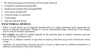
18. • For factor C it is shown in round balls. (High and low values)
• For factor B it is shown in dotted lines (high and low).
Estimating simple effect:
Simple effect of A at low level of B and C=
𝑎
𝑛
−
(1)
𝑛
Simple effect of A at high level of B and low level of C =
𝑎𝑏
𝑛
−
𝑏
𝑛
Simple effect of A at low level of B and high level of C=
𝑎𝑐
𝑛
-
𝑐
𝑛
Simple effect of A at high level of B and C=
𝑎𝑏𝑐
𝑛
−
𝑏𝑐
𝑛
Estimating the main effect:
Main effect of A can be written in short as
• Main effect of A =
𝑎−1 (𝑏−1)(𝑐+1)
4𝑛
a-1 means it should be kept in mind that 1 is given in brackets i.e., [a-(1)].
• Main effect of B =
1
4𝑛
[b+ab+bc+abc-(1)-a-c-ac]

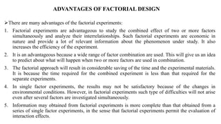
19. In short ,
• Main effect of B =
(𝑎+1)(𝑏−1)(𝑐+1)
4𝑛
• Main effect of C=
1
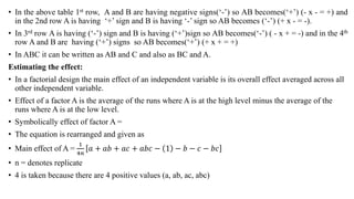
4𝑛
𝑐 + 𝑎𝑐 + 𝑏𝑐 + 𝑎𝑏𝑐 − 1 − 𝑎 − 𝑏 − 𝑎𝑏
• Main effect of c =
(𝑎+1)(𝑏+1)(𝑐−1)
4𝑛
Estimating the interaction effect:
• Interaction effect of AB =
1
4𝑛
[(1)+ab+c+abc-a-b-ac-bc]
In short,
• Interaction of AB =
(𝑎−1)(𝑏−1)(𝑐+1)
4𝑛
• Interaction effect of AC =
1
4𝑛
1 + 𝑏 + 𝑎𝑐 + 𝑎𝑏𝑐 − 𝑎 − 𝑎𝑏 − 𝑐 − 𝑏𝑐
In short,
• Interaction of AC=
(𝑎+1)(𝑏+1)(𝑐−1)
4𝑛
• Interaction effect of BC =
1
4𝑛
[(1)+a+bc+abc-b-ab-c-ac]
In short,
• Interaction of BC=
(𝑎+1)(𝑏−1)(𝑐−1)
4𝑛

20. • Interaction effect of ABC =
1
4𝑛
𝑎𝑏𝑐 + 𝑎 + 𝑏 + 𝑐 − 𝑎𝑏 − 𝑎𝑐 − 𝑏𝑐 − 1
In short,
• Interaction effect of AB=
𝑎−1 (𝑏−1)(𝑐−1)
4𝑛
n= no of replicate
Statistical testing using ANOVA:
Source of variation Sum of squares Df Mean of square f
A SSA 1 MSA =
𝑆𝑆𝐴
1
fA=
𝑀𝑆𝐴
𝑀𝑆𝐸
B SSB 1 MSB=
𝑆𝑆𝐵
1
fB=
𝑀𝑆𝐵
𝑀𝑆𝐸
AB SSAB 1 MSAB=
𝑆𝑆𝐴𝐵
1
fAB=
𝑀𝑆𝐴𝐵
𝑀𝑆𝐸
C SSC 1 MSC=
𝑆𝑆𝐶
1
fc=
𝑀𝑆𝐶
𝑀𝑆𝐸
AC SSAC 1 MSAC=
𝑆𝑆𝐴𝐶
1
fAC=
𝑀𝑆𝐴𝐶
𝑀𝑆𝐸
BC SSBC 1 MSBC=
𝑆𝑆𝐵𝐶
1
fBC=
𝑀𝑆𝐵𝐶
𝑀𝑆𝐸
ABC SSABC 1 MSABC=
𝑆𝑆𝐴𝐵𝐶
1
fABC=
𝑀𝑆𝐴𝐵𝐶
𝑀𝑆𝐸
error SSE 8(n-1) MSE=
𝑆𝑆𝐸
8(𝑛−1)
Total SST 8n-1

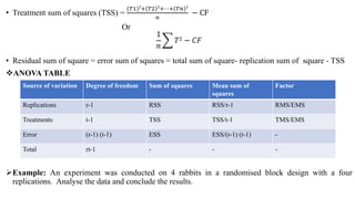
21. • Calculation of sum of squares:
• In the 23 design with n replicates, the sum of squares for any effect is given by
SS=
𝐶𝑜𝑛𝑡𝑟𝑎𝑠𝑡 2
8𝑛
2x2x2=8 [So 8n is taken]
(23)
• Note: The number calculated in the effect of any factors which is inside the bracket is called the
contrast. Also we can take the numerator from the shortcut formula.
For Example:
• Main effect of A =
1
4𝑛
𝑎 + 𝑎𝑏 + 𝑎𝑐 + 𝑎𝑏𝑐 − 1 − 𝑏 − 𝑏𝑐
• The terms which are in bracket are taken as contrast.
In short,
• Main effect of A=
𝑎−1 (𝑏+1)(𝑐+1)
4𝑛
Numerator is contrast.

22. Example:
• A 23 factorial design was used to develop a model for preparing a nanoparticle of optimised size. For
this purpose two concentrations A,B and a powder based drug C were used.
• The experiment is run in 2 replicates and the result is tabulated as follows. The response variable is
the particle size.
Solution:
• Here nanoparticle optimised size is taken as yield.
• A, B taken as liquid.
• C taken as solid.

23. Run A B C Replicate
1
Replicate
2
Total Rotation
1 - - - 550 604 1154 (1)
2 + - - 669 650 1319 a
3 - + - 633 601 1234 b
4 + + - 642 635 1277 ab
5 - - + 1044.5 1044.5 2089 c
6 + - + 749 868 1617 ac
7 - + + 1069 1069 2138 bc
8 - - - 794.5 794.5 1589 abc

24. GRAPHICAL NOTATION
factor minimum maximum
A 1mg/ml 2mg/ml
B o.8mg/ml 1mg/ml
C 30mg 60mg

25. • Estimating the main effect
a = 1319, b = 1234, c = 2089, ab = 1277, ac = 1617, bc = 2138, abc = 1589, (1) = 1154
Main effect of A =
1
4𝑛
𝑎 + 𝑎𝑏 + 𝑎𝑐 + 𝑎𝑏𝑐 − 1 − 𝑏 − 𝑐 − 𝑏𝑐
=
1
8
(1319 + 1277 + 1617 + 1589 − 1154 − 1234 − 2084 − 2138)
=
1
8
(-813) = -101.625
Similarly for B
=
1
4𝑛
𝑏 + 𝑎𝑏 + 𝑏𝑐 + 𝑎𝑏𝑐 − 1 − 𝑎 − 𝑐 − 𝑎𝑐
=
1
8
(1234 + 1277 + 2138 + 1589 − 1154 − 1319 − 2089 − 1617)
=
1
8
(59)
= 7.375

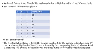
26. • For factor C
=
1
4𝑛
(c +ac + bc + abc- (1) – a-b-ab)
=
1
8
( 2089+1617+2138+ 1589- 1154-1319-1234-1277) =
1
8
( 2449) = 306.125
• Interaction effect of AB
=
1
4𝑛
1 + as + c + abc − a − b − ac − bc
=
1
8
1154 + 1277 + 2089 + 1589 + 1319 − 1234 − 1617 − 2138 = -24.875
• Interaction effect of AC
=
1
4𝑛
1 + 𝑏 + 𝑎𝑐 + 𝑎𝑏𝑐 − 𝑎 − 𝑎𝑏 − 𝑐 − 𝑏𝑐
=
1
8
1154 + 1234 + 1617 + 1589 − 1319 − 1277 − 2089 − 2138
=
1
8
[-1229]
= -153.625

27. • Interaction effect of BC
=
1
4𝑛
[ (1) + a + bc + abc – b – ab – c – ac]
=
1
8
[ 1154 + 1319 + 2138 + 1589 – 1234 -1277 – 2089 – 1617]
=
1
8
[ -17]
= -2.125
• Interaction effect of ABC
=
1
4𝑛
[abc + a + b+ c –ab – ac- bc -1]
=
1
8
[ 1589 + 1319 + 1234+ 2089 – 1277 – 1617-2138 – 1154] =
1
8
[45] = 5.625.
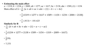
From the calculations
• The largest effects is for
• Factor C = 306.125
• Factor A = -101.625
• AC = -153.625

28. calculate total sum of squares
• SSA =
−813 2
16
=
𝑐𝑜𝑛𝑡𝑟𝑎𝑠𝑡 2
8𝑛
= 41310.5625 since here 2 replicates are there 8 x 2 = 16
• SSB =
59 2
16
= 217.5625
• SSC =
2449 2
16
= 374850.0625
• SSAB =
−199 2
16
= 2475.0625
• SSAC =
−1229 2
16
= 94402.5625
• SSBC =
−17 2
16
= 18.0625
• SSABC =
45 2
16
= 126.5625

29. From the table we find that factor A and factor C are highly significant. And the interaction AC is highly
significant .
So there is a strong interaction between factor A and factor C.
Note: Factorial design can be done using regression also.
Source of
variation
Sum of squares DF Mean square F P value
A 41310.5625 1 41310.5625 18.34 0.0027
B 217.5625 1 217.5625 0.10 0.7639
C 374850.0625 1 374850.0625 166.41 0.0001
AB 2475.0625 1 2475.0625 1.10 0.5252
AC 94402.5625 1 94402.5625 41.91 0.0002
BC 18.0625 1 18.0625 0.01 0.9308
ABC 126.5625 1 126.5625 0.06 0.8186
Error 18020.5000 8 2252.5625
Total 531420.9375 15