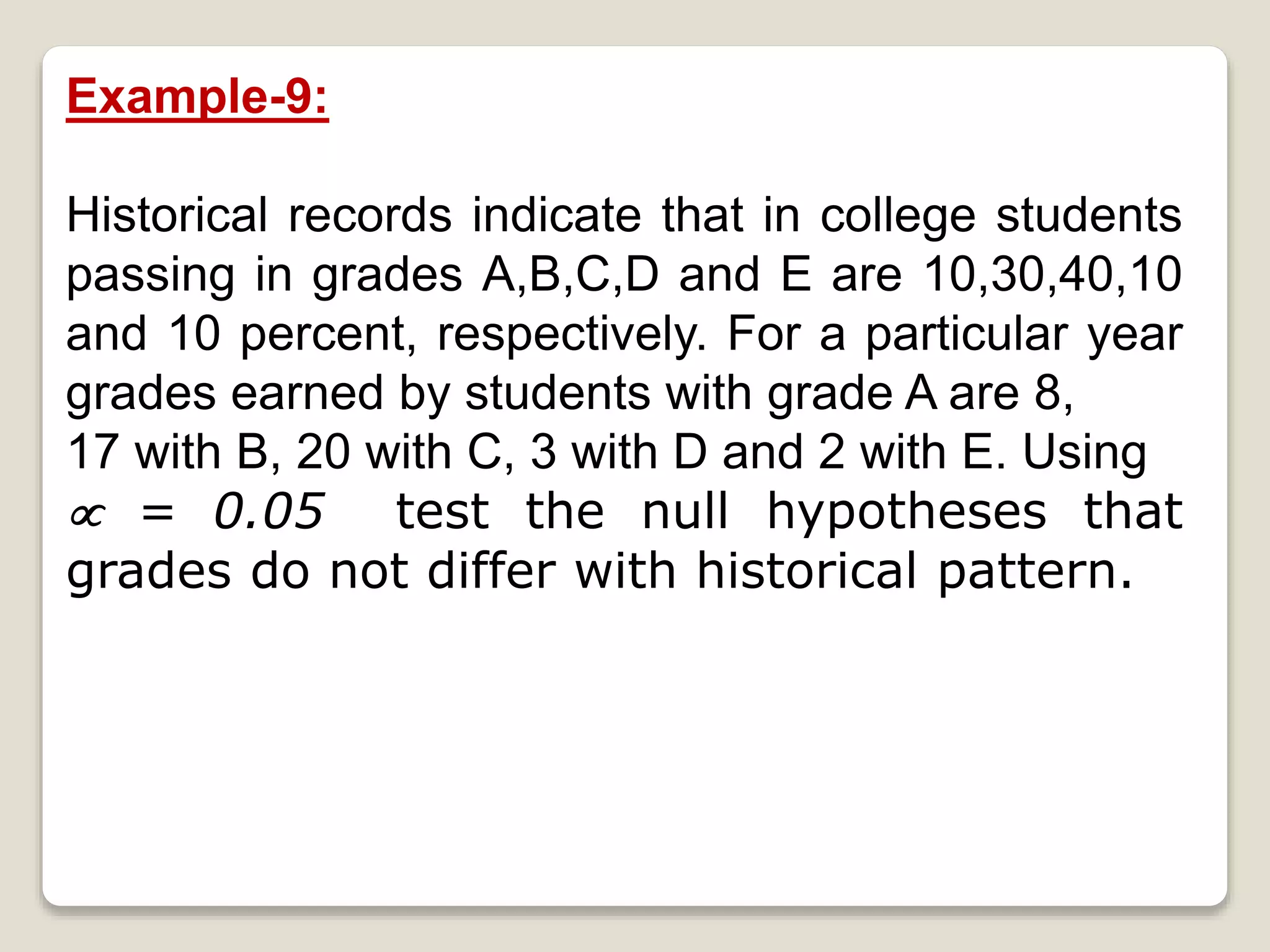
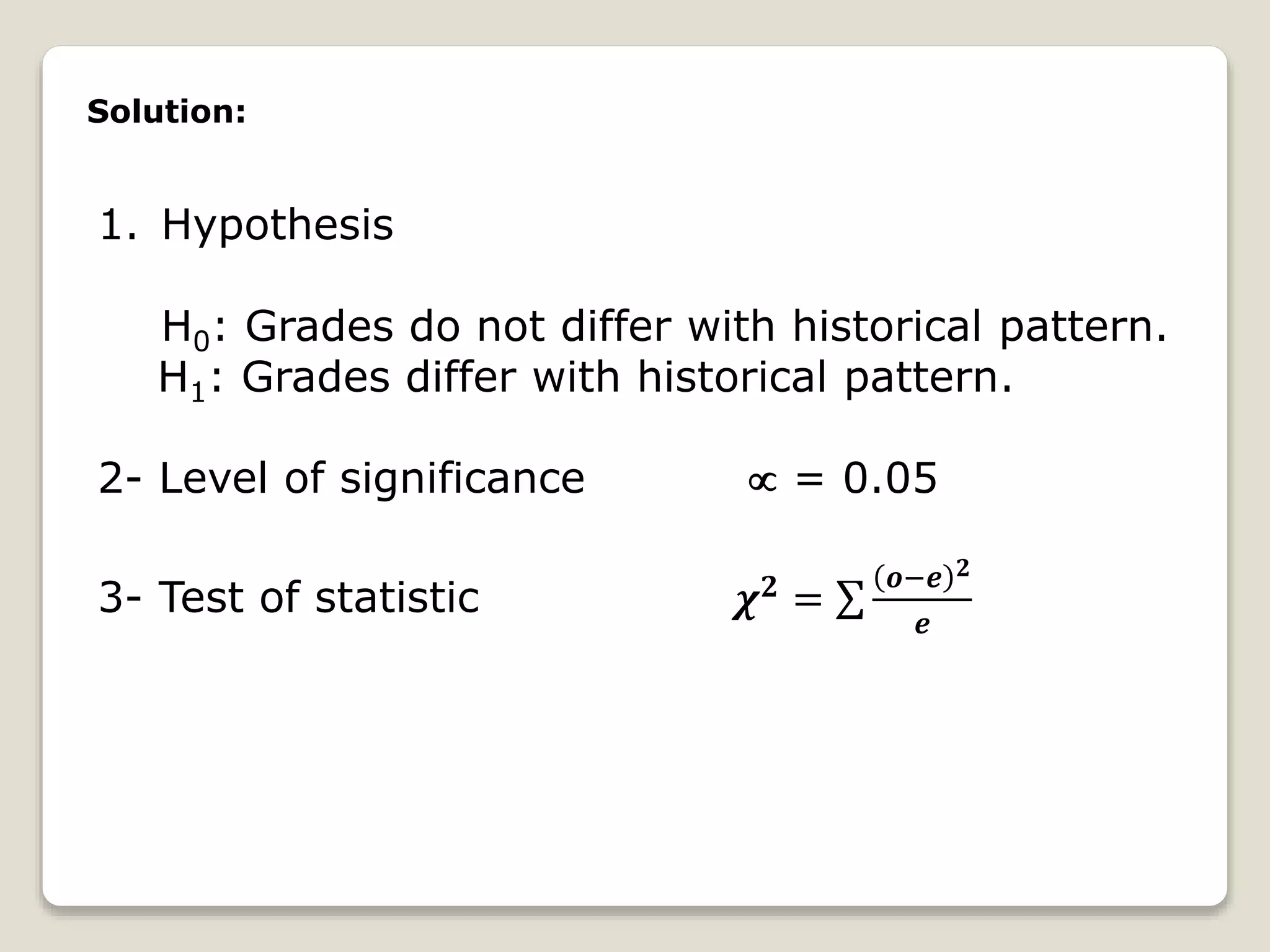
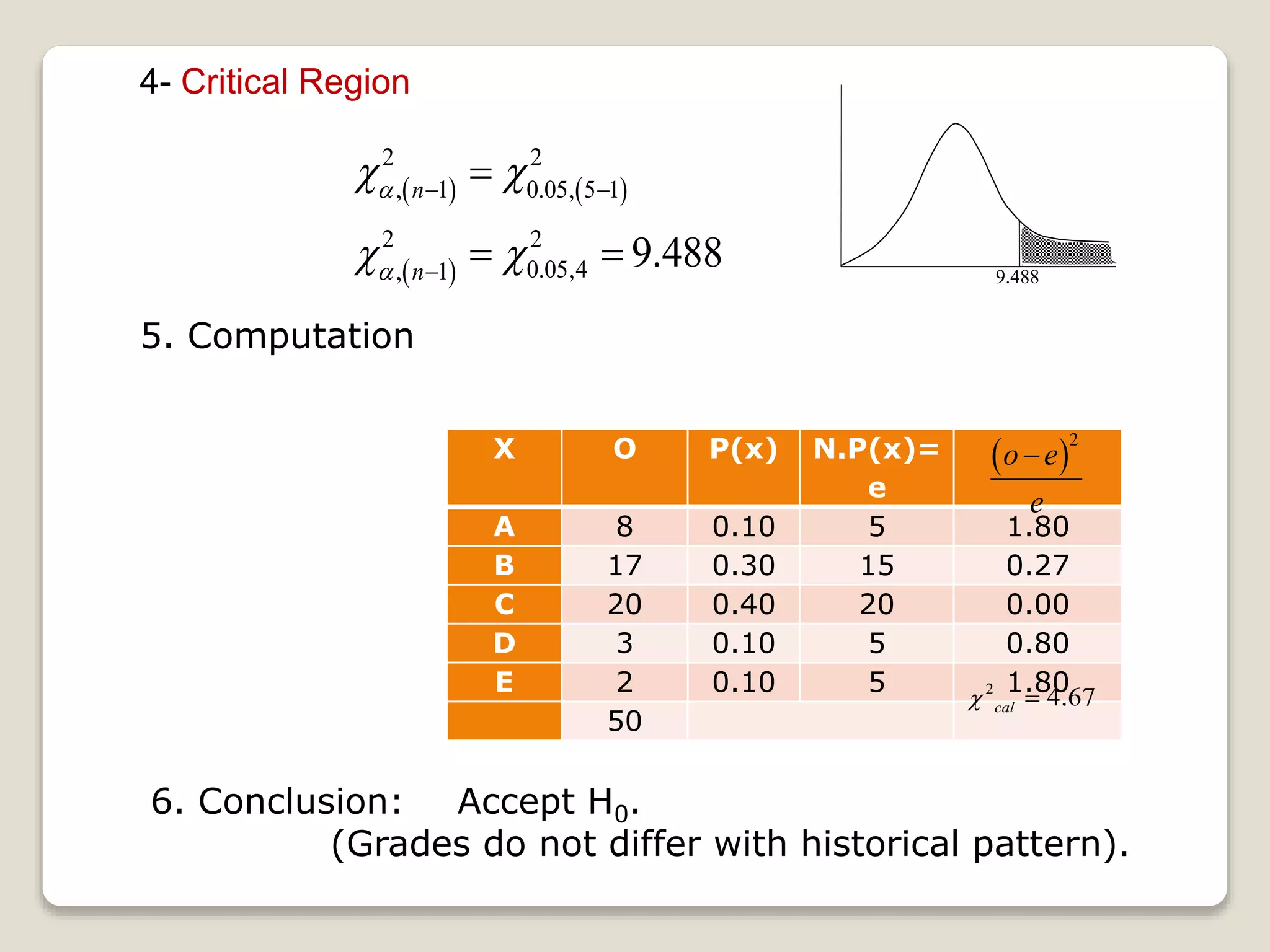
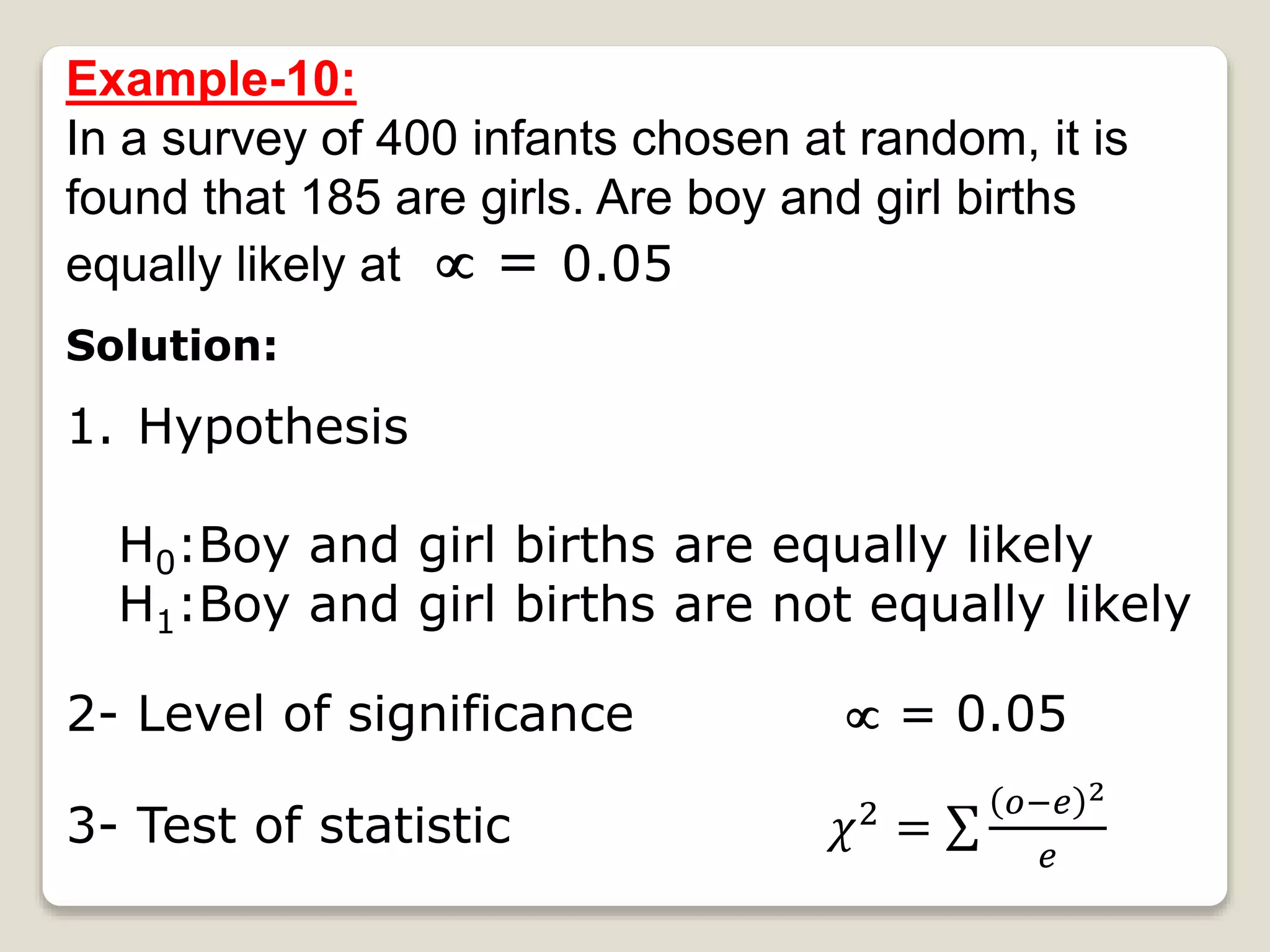
1. This document discusses procedures for conducting chi-square goodness of fit and independence tests. 2. Chi-square goodness of fit tests are used to determine if sample data fits a hypothesized distribution. Chi-square tests for independence examine whether two categorical variables are associated. 3. The tests involve defining hypotheses, determining significance levels, calculating test statistics, finding critical values, performing computations, and making conclusions about whether to reject or fail to reject the null hypothesis.

1. HYPOTHESIS TESTING
PART-I
NADEEM UDDIN
ASSOCIATE PROFESSOR
OF STATISTICS

2. Chi-Square Goodness of Fit Test:
This lesson explains how to conduct a chi-
square goodness of fit test. The test is
applied when you have one categorical
variable from a single population. It is
used to determine whether sample data
are consistent with a hypothesized
distribution.

3. Procedure Goodness of fit test
1-Hypothesis H0: Fit is good.
H1: Fit is not good.
2-Level of significance  = 1% or 5% or
any given value.
3-Test of statistic 𝜒2 =
𝑜−𝑒 2
𝑒
Where o = observed value
e = estimated value

4. 4-Critical region 𝜒2
, 𝑛−1
5- Computation
6-Conclusion
If the calculated value of test
statistic falls in the area of
rejection, we reject the null
hypothesis otherwise accept it.

5. Example-8:
To investigate whether the following
distribution of grades is uniform at 5%
level of significance.
Grades A B C D E
F 25 30 22 32 15

6. Solution:
1- Hypothesis H0: Distribution of grades is uniform.
H1:Distribution of grades is not uniform.
2- Level of significance  = 0.05
3- Test of statistic 𝝌 𝟐
=
𝒐−𝒆 𝟐
𝒆
4- Critical region    
 
2 2
, 1 0.05, 5 1
2 2
0.05,4, 1
9.488
n
n


 
 
 


 
9.488

7. 5. Computation
X O P(x) N.P(x)=
e
A 25 1/5 24.8 0.0016
B 30 1/5 24.8 1.0903
C 22 1/5 24.8 0.3161
D 32 1/5 24.8 2.0903
E 15 1/5 24.8 3.8726
124
 
2
o e
e

2
7.371cal 
6. Conclusion: Accept H0.
(Distribution of grades is uniform)

8. Example-9:
Historical records indicate that in college students
passing in grades A,B,C,D and E are 10,30,40,10
and 10 percent, respectively. For a particular year
grades earned by students with grade A are 8,
17 with B, 20 with C, 3 with D and 2 with E. Using
 = 0.05 test the null hypotheses that
grades do not differ with historical pattern.

9. Solution:
1. Hypothesis
H0: Grades do not differ with historical pattern.
H1: Grades differ with historical pattern.
2- Level of significance  = 0.05
3- Test of statistic 𝝌 𝟐 =
𝒐−𝒆 𝟐
𝒆

10.    
 
2 2
, 1 0.05, 5 1
2 2
0.05,4, 1
9.488
n
n


 
 
 


  9.488
4- Critical Region
5. Computation
6. Conclusion: Accept H0.
(Grades do not differ with historical pattern).
X O P(x) N.P(x)=
e
A 8 0.10 5 1.80
B 17 0.30 15 0.27
C 20 0.40 20 0.00
D 3 0.10 5 0.80
E 2 0.10 5 1.80
50
 
2
o e
e

2
4.67cal 

11. Example-10:
In a survey of 400 infants chosen at random, it is
found that 185 are girls. Are boy and girl births
equally likely at  = 0.05
Solution:
1. Hypothesis
H0:Boy and girl births are equally likely
H1:Boy and girl births are not equally likely
2- Level of significance  = 0.05
3- Test of statistic 𝜒2 =
𝑜−𝑒 2
𝑒

12. 4. Critical Region
2
 α,(n-1) =
2
 0.05,(2-1)
2
 0.05,1 = 3.841
5. Computation
X O P(x) N.P(x)
=e
Girls 185 ½ 200 1.125
Boys 215 ½ 200 1.125
400
 
2
o e
e

2
2.250cal 
6. Conclusion: Accept H0.

13. Chi-Square Test for Independence:
This lesson explains how to conduct a chi-
square test for independence. The test is
applied when you have two categorical
variables from a single population. It is
used to determine whether there is a
significant association between the two
variables.

14. Procedure Test Concerning for independence
1-Hypothesis
H0: The two attributes are not associated.
H1: The two attributes are associated.
2-Level of significance  = 1% or 5% or any given
value.
3-Test of statistic 𝝌 𝟐 =
𝒐−𝒆 𝟐
𝒆
Where o = observed value
e = estimated value

15. 4-Critical region 𝜒2
, 𝑟−1 (𝑐−1)
5-Computation
6-Conclusion
If the calculated value of test statistic
falls in the area of rejection, we reject
the null hypothesis otherwise accept it.

16. Weather
Total
Good Bad
Result
Win 12 4 16
Draw 5 8 13
Lose 7 14 21
Total 24 26 50
Example-11:
The members of a sports team are interested in
whether the weather has an effect on their results.
They play 50 matches, with the following results:
Test the claim at 1% significance level that
the result independent of weather.

17. Solution:
1-Hypothesis
H0: Result independent of weather.
H1: Result dependent of weather.
2- Level of significance  = 0.01
3- Test of statistic 𝜒2
=
𝑜−𝑒 2
𝑒

18. 4. Critical Region
𝜒2
, 𝑟−1 (𝑐−1)
𝜒2
0.01, 3−1 (2−1)
𝜒2
,2 = 9.21 9.21

19. 5. Computation
Good Bad Total
Win 12
24 × 16
50
= 7.68
4
26 × 16
50
= 8.32 16
Dra
w
5
13 × 24
50
= 6.24 8
26 × 13
50
= 6.76 13
Loos
e
7
24 × 21
50
= 10.08
14
26 × 21
50
= 10.92
21
Total 24 26 50

20. O e
12 7.68 2.43
5 6.24 0.246
7 10.08 0.941
4 8.32 2.243
8 6.76 0.227
14 10.92 0.868
 
2
o e
e

2
6.956cal 
6. Conclusion:
Accept H0.
And conclude that the team’s
result are independent of the weather.