This document discusses inventory management concepts including the costs associated with holding too much inventory, different inventory control systems, determining reorder points and economic order quantities, quantity discounts, and using safety stock. It provides examples to demonstrate how to calculate the optimal order quantity using the economic order quantity model, determining reorder points, applying the economic production quantity model, analyzing quantity discount schedules, and determining appropriate safety stock levels.

1. Course: MBA
Subject: Production & Operation
Management
Unit:3.1
Inventory Management

2. Inventory Management
• When you keep too much inventory on hand, the
cost of inventory can increase by as much as 25
percent. Added costs include:
financing
opportunity
storage
insurance
shrinkage
obsolescence

3. Various cost
• Financing cost on excess inventory can impact
the prices businesses charge customers.
• financing cost the cost of interest paid to
borrow money
• A business can incur opportunity cost and
storage cost by keeping too much inventory.
• opportunity cost the cost associated with giving
up the use of money tied up in inventory
• storage cost the cost associated with renting or
buying space needed to store inventory

4. Various cost
• A business with sound inventory procedures
can reduce insurance cost and shrinkage cost.
• insurance cost the cost associated with
insuring inventory
• shrinkage cost the cost associated with the
loss of inventory items that are broken,
damaged, spoiled, or stolen

5. • A business must closely monitor inventory
turnover rates in order to control
obsolescence cost on items that remain in
inventory too long.
• obsolescence cost the cost associated with
products or materials that become obsolete
while in inventory

6. Planning Inventory
• There are two steps involved in determining
the amount of inventory you need:
1. Calculate the supply you need.
2. Calculate the inventory investment.

7. Inventory Control
• Inventory control systems include:
visual inventory system
perpetual inventory system
partial inventory system
just-in-time (JIT) inventory system

8. Warehousing
• Warehousing operations can occur in
dedicated structure or an assigned space
within a structure.
• warehousing the act of holding and handling
goods in a warehouse

9. Warehouse Operations Areas
Picking
rows
Receiving and
shipping docks
Bulk storage areas
Management
office and
lockers
Staging
areas
Assembly
areas
Packing
areas

10. Reordering
To maintain proper inventory levels, you need
to decide when and how much to reorder.
The type of inventory you keep determines
which reordering system is best for you:
periodic reordering
nonperiodic reordering

11. Reordering
Products or raw materials that are inexpensive,
used often, and easy to get should be reordered
periodically.
A sandwich shop might restock bread daily.
Lead time must be considered for inventory
that is suited to nonperiodic reordering.
lead time the gap in time between placing an
order and receiving delivery

12. Reordering
• When using a nonperiodic reordering system,
inventory needs must be projected so that usage
rate can be calculated and safety stock is
available.
• usage rate how quickly inventory will be used in
a given period of time
• safety stock a cushion of products or materials
that prevents a business from running out of
inventory while waiting for an order

13. Economic Order Quantity (EOQ):
Determining How Much to Order
• One of the oldest and most well known
inventory control techniques
• Easy to use
• Based on a number of assumptions

14. Assumptions of the EOQ Model
1. Demand is known and constant
2. Lead time is known and constant
3. Receipt of inventory is instantaneous
4. Quantity discounts are not available
5. Variable costs are limited to: ordering cost
and carrying (or holding) cost
6. If orders are placed at the right time,
stockouts can be avoided

15. Inventory Level Over Time
Based on EOQ Assumptions

16. Minimizing EOQ Model Costs
• Only ordering and carrying costs need to be
minimized (all other costs are assumed
constant)
• As Q (order quantity) increases:
–Carry cost increases
–Ordering cost decreases (since the number
of orders per year decreases)

17. EOQ Model Total Cost
At optimal order quantity (Q*):
Carrying cost = Ordering cost

18. Finding the Optimal Order Quantity
Parameters:
Q* = Optimal order quantity (the EOQ)
D = Annual demand
Co = Ordering cost per order
Ch = Carrying (or holding) cost per unit per yr
P = Purchase cost per unit

19. Two Methods for Carrying Cost
Carry cost (Ch) can be expressed either:
1. As a fixed cost, such as
Ch = $0.50 per unit per year
2. As a percentage of the item’s purchase cost
(P)
Ch = I x P
I = a percentage of the purchase cost

20. EOQ Total Cost
Total ordering cost = (D/Q) x Co
Total carrying cost = (Q/2) x Ch
Total purchase cost = P x D
= Total cost
Note:
• (Q/2) is the average inventory level
• Purchase cost does not depend on Q

21. Finding Q*
Recall that at the optimal order quantity (Q*):
Carry cost = Ordering cost
(D/Q*) x Co = (Q*/2) x Ch
Rearranging to solve for Q*:
Q* = )/2( hCDCo

22. EOQ Example: Sumco Pump Co.
Buys pump housing from a manufacturer and
sells to retailers
D = 1000 pumps annually
Co = $10 per order
Ch = $0.50 per pump per year
P = $5
Q* = ?

23. Using ExcelModules for Inventory
• Worksheet for inventory models in
ExcelModules are color coded
– Input cells are yellow
– Output cells are green
• Select “Inventory Models” from the
ExcelModules menu, then select “EOQ”
Go to file 12-2.xls

24. Average Inventory Value
After Q* is found we can calculate the average
value of inventory on hand
Average inventory value = P x (Q*/2)

25. Calculating Ordering and
Carrying Costs for a Given Q
• Sometimes Co and Ch are difficult to estimate
• We can use the EOQ formula to calculate the
value of Co or Ch that would make a given Q
optimal:
Co = Q2 x Ch/(2D)
Ch = 2DCo/Q2

26. Sensitivity of the EOQ Formula
• The EOQ formula assumes all inputs are know
with certainty
• In reality these values are often estimates
• Determining the effect of input value changes
on Q* is called sensitivity analysis

27. Sensitivity Analysis for Sumco
• Suppose Co = $15 (instead of $10), which is a
50% increase
• Assume all other values are unchanged
• The new Q* = 245 (instead of 200), which is a
22.5% increase
• This shows the nonlinear nature of the
formula

28. Reorder Point:
Determining When to Order
• After Q* is determined, the second decision is
when to order
• Orders must usually be placed before
inventory reaches 0 due to order lead time
• Lead time is the time from placing the order
until it is received
• The reorder point (ROP) depends on the lead
time (L)

29. Reorder Point (ROP)
ROP = d x L

30. Sumco Example Revisited
• Assume lead time, L = 3 business days
• Assume 250 business days per year
• Then daily demand,
d = 1000 pumps/250 days = 4 pumps per day
ROP = (4 pumps per day) x (3 days)
= 12 pumps
Go to file 12-3.xls

31. Economic Production Quantity:
Determining How Much to Produce
• The EOQ model assumes inventory arrives
instantaneously
• In many cases inventory arrives gradually
• The economic production quantity (EPQ)
model assumes inventory is being produced at
a rate of p units per day
• There is a setup cost each time production
begins

32. Inventory Control With Production

33. Determining Lot Size or EPQ
Parameters
Q* = Optimal production quantity (or EPQ)
Cs = Setup cost
D = annual demand
d = daily demand rate
p = daily production rate

34. Average Inventory Level
• We will need the average inventory level for
finding carrying cost
• Average inventory level is ½ the maximum
Max inventory = Q x (1- d/p)
Ave inventory = ½ Q x (1- d/p)

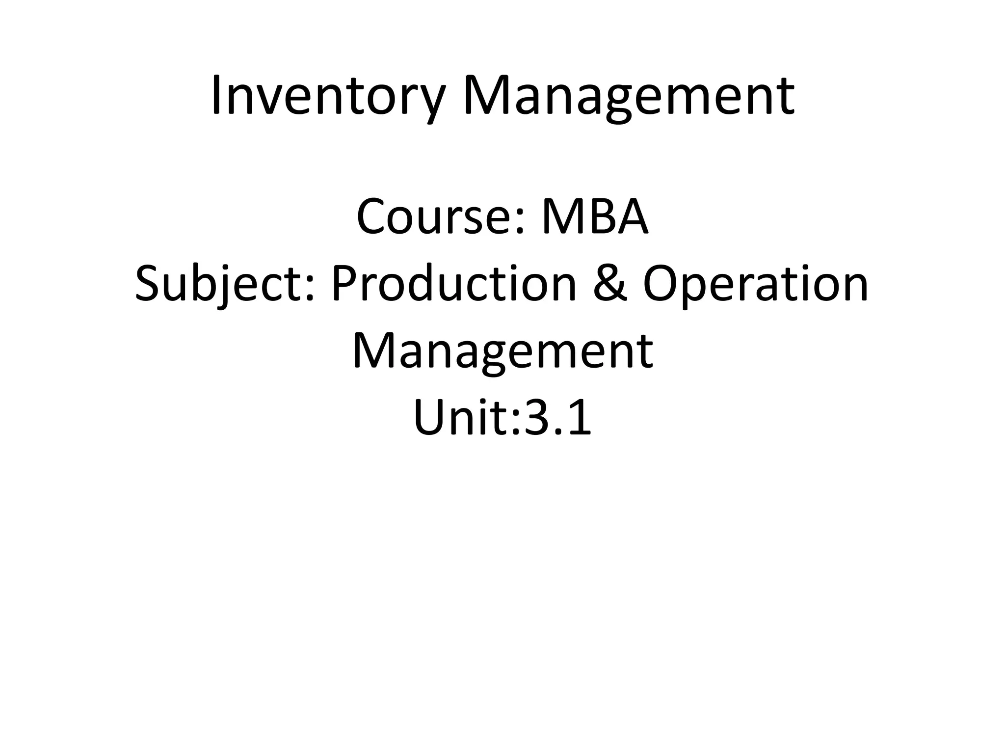
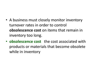
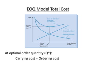
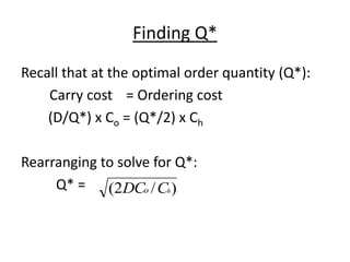
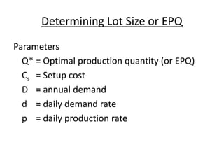
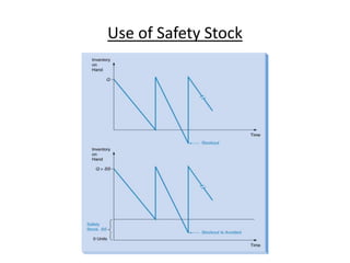
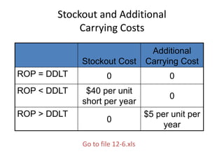
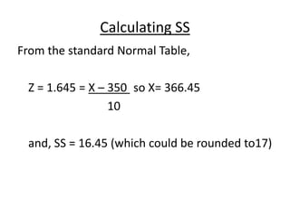
35. Total Cost
Setup cost = (D/Q) x Cs
Carrying cost = [½ Q x (1- d/p)] x Ch
Production cost = P x D
= Total cost
As in the EOQ model:
• The production cost does not depend on Q
• The function is nonlinear

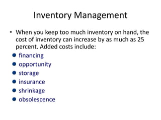
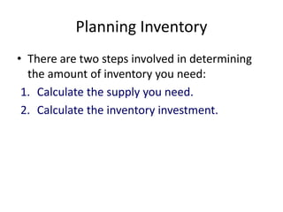
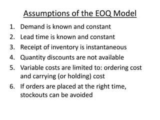
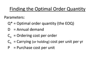
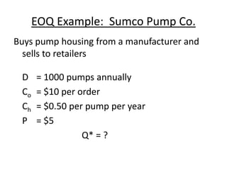
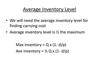
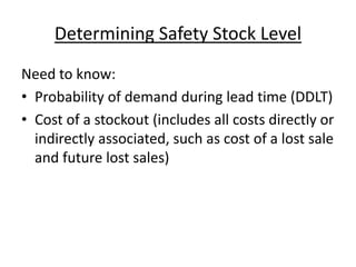
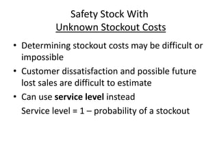
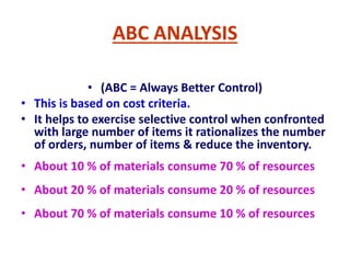
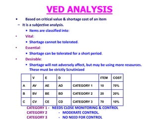
36. Finding Q*
• As in the EOQ model, at the optimal quantity Q*
we should have:
Setup cost = Carrying cost
(D/Q*) x Cs = [½ Q* x (1- d/p)] x Ch
Rearranging to solve for Q*:
Q* = )]/1(/[2( pdCDC hs 

37. EPQ for Brown Manufacturing
Produces mini refrigerators (has 167 business
days per year)
D = 10,000 units annually
d = 1000 / 167 = ~60 units per day
p = 80 units per day (when producing)
Ch = $0.50 per unit per year
Cs = $100 per setup
P = $5 to produce each unit
Go to file 12-4.xls

38. Length of the Production Cycle
• The production cycle will last until Q* units
have been produced
• Producing at a rate of p units per day means
that it will last (Q*/p) days
• For Brown this is:
Q* = 4000 units
p = 80 units per day
4000 / 80 = 50 days

39. Quantity Discount Models
• A quantity discount is a reduced unit price based
on purchasing a large quantity
• Example discount schedule:

40. Four Steps to Analyze
Quantity Discount Models
1. Calculate Q* for each discount price
2. If Q* is too small to qualify for that price,
adjust Q* upward
3. Calculate total cost for each Q*
4. Select the Q* with the lowest total cost

41. Brass Department Store Example
Sells toy cars
D = 5000 cars annually
Co = $49 per order
Ch = $0.20 per car per year
Quantity Discount Schedule
go to file 12-5.xls

42. Use of Safety Stock
• Safety stock (SS) is extra inventory held to
help prevent stockouts
• Frequently demand is subject to random
variability (uncertainty)
• If demand is unusually high during lead time,
a stockout will occur if there is no safety stock

43. Use of Safety Stock

44. Determining Safety Stock Level
Need to know:
• Probability of demand during lead time (DDLT)
• Cost of a stockout (includes all costs directly or
indirectly associated, such as cost of a lost sale
and future lost sales)

45. ABCO Safety Stock Example
• ROP = 50 units (from previous EOQ)
• Place 6 orders per year
• Stockout cost per unit = $40
• Ch = $5 per unit per year
• DDLT has a discrete distribution

46. Analyzing the Alternatives
• With uncertain DDLT this becomes a “decision
making under risk” problem
• Each of the five possible values of DDLT
represents a decision alternative for ROP
• Need to determine the economic payoff for
each combination of decision alternative
(ROP) and outcome (DDLT)

47. Stockout and Additional
Carrying Costs
Stockout Cost
Additional
Carrying Cost
ROP = DDLT 0 0
ROP < DDLT $40 per unit
short per year
0
ROP > DDLT
0
$5 per unit per
year
Go to file 12-6.xls

48. Safety Stock With
Unknown Stockout Costs
• Determining stockout costs may be difficult or
impossible
• Customer dissatisfaction and possible future
lost sales are difficult to estimate
• Can use service level instead
Service level = 1 – probability of a stockout

49. Hinsdale Co. Example
• DDLT follows a normal distribution
(μ = 350, σ = 10)
• They want a 95% service level (i.e. 5%
probability of a stockout)
SS = ?

50. Safety Stock and the Normal Distribution

51. Calculating SS
From the standard Normal Table,
Z = 1.645 = X – 350 so X= 366.45
10
and, SS = 16.45 (which could be rounded to17)

52. ABC ANALYSIS
• (ABC = Always Better Control)
• This is based on cost criteria.
• It helps to exercise selective control when confronted
with large number of items it rationalizes the number
of orders, number of items & reduce the inventory.
• About 10 % of materials consume 70 % of resources
• About 20 % of materials consume 20 % of resources
• About 70 % of materials consume 10 % of resources

53. ‘A’ ITEMS
– Small in number, but consume large amount of
resources
– Must have:
• Tight control
• Rigid estimate of requirements
• Strict & closer watch
• Low safety stocks
• Managed by top management

54. ‘B’ ITEM
• Intermediate
• Must have:
• Moderate control
• Purchase based on rigid requirements
• Reasonably strict watch & control
• Moderate safety stocks
• Managed by middle level management

55. ‘C’ ITEMS
• Larger in number, but consume lesser
amount of resources
• Must have:
• Ordinary control measures
• Purchase based on usage estimates
• High safety stocks
• ABC analysis does not stress on items those are less
costly but may be vital

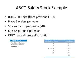
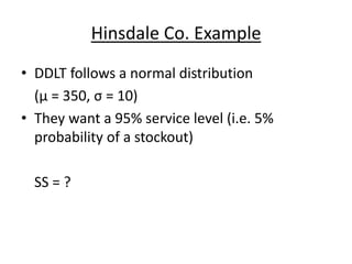
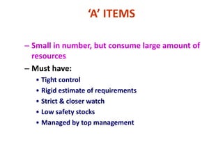
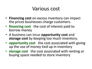
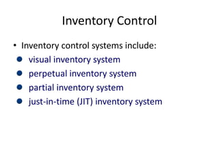
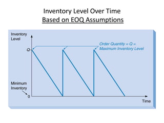
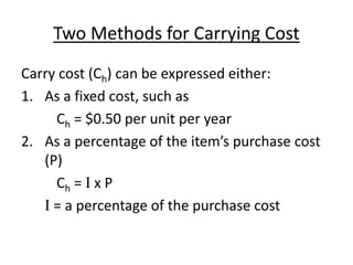
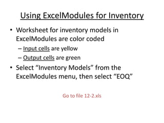
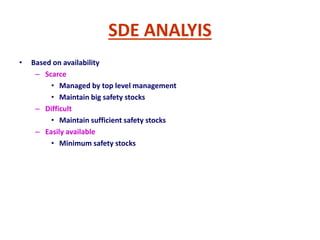
56. 20000050020
19950050019
19900050018
19850050017
19800050016
19750050015
19700050014
19650050013
196000150012
194500150011
193000175010
19125027509
18850040008
18450045007
18000050006
17500075005
16750075004
160000200003
140000500002
90000900001
CUMMULATIVECUMMULATIVE
COSTCOST [Rs.]
ANNUAL COSTANNUAL COST
[Rs.]
ITEMITEM COST %COST %ITEM %ITEM %
70 %70 %
20 %20 %
10 %10 %
10 %10 %
20 %20 %
70 %70 %
ABC
A
N
A
L
Y
S
I
S
WORK
SHEET

57. VED ANALYSIS
• Based on critical value & shortage cost of an item
– It is a subjective analysis.
• Items are classified into:
• Vital:
• Shortage cannot be tolerated.
• Essential:
• Shortage can be tolerated for a short period.
• Desirable:
 Shortage will not adversely affect, but may be using more resources.
These must be strictly Scrutinized
V E D ITEM COST
A AV AE AD CATEGORY 1 10 70%
B BV BE BD CATEGORY 2 20 20%
C CV CE CD CATEGORY 3 70 10%
CATEGORY 1 - NEEDS CLOSE MONITORING & CONTROL
CATEGORY 2 - MODERATE CONTROL.
CATEGORY 3 - NO NEED FOR CONTROL

58. SDE ANALYIS
• Based on availability
– Scarce
• Managed by top level management
• Maintain big safety stocks
– Difficult
• Maintain sufficient safety stocks
– Easily available
• Minimum safety stocks

59. FSN ANALYSIS
– Based on utilization.
– Fast moving.
– Slow moving.
– Non-moving.
– Non-moving items must be periodically reviewed to prevent expiry
– & obsolescence

60. HML ANALYSIS
• Based on cost per unit
• Highest
• Medium
• Low
• This is used to keep control over
consumption at departmental level for
deciding the frequency of physical
verification.

61. Reference
• www.pitt.edu
• www.caal-inteduorg.com
• https://www.scribd.com