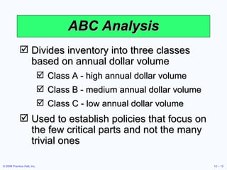
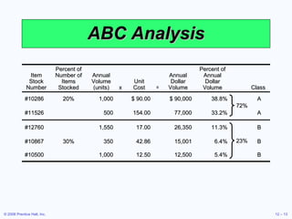
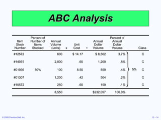
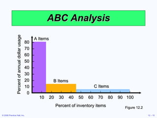
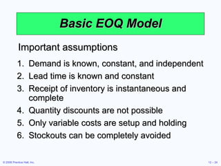
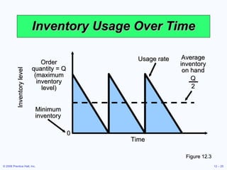
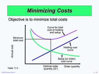
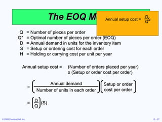
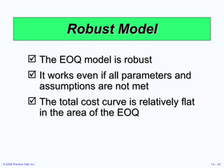
This document discusses inventory management concepts and models. It begins by outlining learning objectives related to ABC analysis, cycle counting, economic order quantity (EOQ) models, reorder points, and other topics. It then provides details on Amazon's inventory management practices and types of inventory. The bulk of the document explains ABC analysis for classifying inventory, techniques for maintaining accurate records, factors that influence holding and ordering costs, and the EOQ model for determining optimal order quantities. It concludes by noting the robustness of the EOQ model and introducing the concept of reorder points.

1. Operations Management Session 6 – Inventory Management

2. Learning Objectives When you complete this chapter you should be able to: Conduct an ABC analysis Explain and use cycle counting Explain and use the EOQ model for independent inventory demand Compute a reorder point and safety stock

3. Learning Objectives When you complete this chapter you should be able to: Apply the production order quantity model Explain and use the quantity discount model Understand service levels and probabilistic inventory models

4. Amazon.com Amazon.com started as a “virtual” retailer – no inventory, no warehouses, no overhead; just computers taking orders to be filled by others Growth has forced Amazon.com to become a world leader in warehousing and inventory management

5. Amazon.com Each order is assigned by computer to the closest distribution center that has the product(s) A “flow meister” at each distribution center assigns work crews Lights indicate products that are to be picked and the light is reset Items are placed in crates on a conveyor. Bar code scanners scan each item 15 times to virtually eliminate errors.

6. Amazon.com Crates arrive at central point where items are boxed and labeled with new bar code Gift wrapping is done by hand at 30 packages per hour Completed boxes are packed, taped, weighed and labeled before leaving warehouse in a truck Order arrives at customer within a week

7. Inventory One of the most expensive assets of many companies representing as much as 50% of total invested capital Operations managers must balance inventory investment and customer service

8. Functions of Inventory To decouple or separate various parts of the production process To decouple the firm from fluctuations in demand and provide a stock of goods that will provide a selection for customers To take advantage of quantity discounts To hedge against inflation

9. Types of Inventory Raw material Purchased but not processed Work-in-process Undergone some change but not completed A function of cycle time for a product Maintenance/repair/operating (MRO) Necessary to keep machinery and processes productive Finished goods Completed product awaiting shipment

10. The Material Flow Cycle Figure 12.1 Input Wait for Wait to Move Wait in queue Setup Run Output inspection be moved time for operator time time Cycle time 95% 5%

11. Inventory Management How inventory items can be classified How accurate inventory records can be maintained

12. ABC Analysis Divides inventory into three classes based on annual dollar volume Class A - high annual dollar volume Class B - medium annual dollar volume Class C - low annual dollar volume Used to establish policies that focus on the few critical parts and not the many trivial ones

13. ABC Analysis Item Stock Number Percent of Number of Items Stocked Annual Volume (units) x Unit Cost = Annual Dollar Volume Percent of Annual Dollar Volume Class #10286 20% 1,000 $ 90.00 $ 90,000 38.8% A #11526 500 154.00 77,000 33.2% A #12760 1,550 17.00 26,350 11.3% B #10867 30% 350 42.86 15,001 6.4% B #10500 1,000 12.50 12,500 5.4% B 72% 23%

14. ABC Analysis Item Stock Number Percent of Number of Items Stocked Annual Volume (units) x Unit Cost = Annual Dollar Volume Percent of Annual Dollar Volume Class #12572 600 $ 14.17 $ 8,502 3.7% C #14075 2,000 .60 1,200 .5% C #01036 50% 100 8.50 850 .4% C #01307 1,200 .42 504 .2% C #10572 250 .60 150 .1% C 8,550 $232,057 100.0% 5%

15. ABC Analysis Figure 12.2 A Items B Items C Items Percent of annual dollar usage 80 – 70 – 60 – 50 – 40 – 30 – 20 – 10 – 0 – | | | | | | | | | | 10 20 30 40 50 60 70 80 90 100 Percent of inventory items

16. ABC Analysis Other criteria than annual dollar volume may be used Anticipated engineering changes Delivery problems Quality problems High unit cost

17. ABC Analysis Policies employed may include More emphasis on supplier development for A items Tighter physical inventory control for A items More care in forecasting A items

18. Record Accuracy Accurate records are a critical ingredient in production and inventory systems Allows organization to focus on what is needed Necessary to make precise decisions about ordering, scheduling, and shipping Incoming and outgoing record keeping must be accurate Stockrooms should be secure

19. Control of Service Inventories Can be a critical component of profitability Losses may come from shrinkage or pilferage Applicable techniques include Good personnel selection, training, and discipline Tight control on incoming shipments Effective control on all goods leaving facility

20. Holding, Ordering, and Setup Costs Holding costs - the costs of holding or “carrying” inventory over time Ordering costs - the costs of placing an order and receiving goods Setup costs - cost to prepare a machine or process for manufacturing an order

21. Holding Costs Table 12.1 Category Cost (and range) as a Percent of Inventory Valu e Housing costs (building rent or depreciation, operating costs, taxes, insurance) 6% (3 - 10%) Material handling costs (equipment lease or depreciation, power, operating cost) 3% (1 - 3.5%) Labor cost 3% (3 - 5%) Investment costs (borrowing costs, taxes, and insurance on inventory) 11% (6 - 24%) Pilferage, space, and obsolescence 3% (2 - 5%) Overall carrying cost 26%

22. Holding Costs Table 12.1 Category Cost (and range) as a Percent of Inventory Valu e Housing costs (building rent or depreciation, operating costs, taxes, insurance) 6% (3 - 10%) Material handling costs (equipment lease or depreciation, power, operating cost) 3% (1 - 3.5%) Labor cost 3% (3 - 5%) Investment costs (borrowing costs, taxes, and insurance on inventory) 11% (6 - 24%) Pilferage, space, and obsolescence 3% (2 - 5%) Overall carrying cost 26% Holding costs vary considerably depending on the business, location, and interest rates. Generally greater than 15%, some high tech items have holding costs greater than 50%.

23. Inventory Models for Independent Demand Basic economic order quantity Production order quantity Quantity discount model Need to determine when and how much to order

24. Basic EOQ Model Demand is known, constant, and independent Lead time is known and constant Receipt of inventory is instantaneous and complete Quantity discounts are not possible Only variable costs are setup and holding Stockouts can be completely avoided Important assumptions

25. Inventory Usage Over Time Figure 12.3 Order quantity = Q (maximum inventory level) Usage rate Average inventory on hand Q 2 Minimum inventory Inventory level Time 0

26. Minimizing Costs Objective is to minimize total costs Table 11.5 Annual cost Order quantity Curve for total cost of holding and setup Holding cost curve Setup (or order) cost curve Minimum total cost Optimal order quantity (Q*)

27. The EOQ Model Q = Number of pieces per order Q* = Optimal number of pieces per order (EOQ) D = Annual demand in units for the inventory item S = Setup or ordering cost for each order H = Holding or carrying cost per unit per year Annual setup cost = (Number of orders placed per year) x (Setup or order cost per order) Annual demand Number of units in each order Setup or order cost per order = Annual setup cost = S D Q = (S) D Q

28. The EOQ Model Q = Number of pieces per order Q* = Optimal number of pieces per order (EOQ) D = Annual demand in units for the inventory item S = Setup or ordering cost for each order H = Holding or carrying cost per unit per year Annual holding cost = (Average inventory level) x (Holding cost per unit per year) Order quantity 2 = (Holding cost per unit per year) = (H) Q 2 Annual setup cost = S D Q Annual holding cost = H Q 2

29. The EOQ Model Q = Number of pieces per order Q* = Optimal number of pieces per order (EOQ) D = Annual demand in units for the inventory item S = Setup or ordering cost for each order H = Holding or carrying cost per unit per year Optimal order quantity is found when annual setup cost equals annual holding cost Solving for Q* Annual setup cost = S D Q Annual holding cost = H Q 2 D Q S = H Q 2 2DS = Q 2 H Q 2 = 2DS/H Q* = 2DS/H

30. An EOQ Example Determine optimal number of needles to order D = 1,000 units S = $10 per order H = $.50 per unit per year Q* = 2DS H Q* = 2(1,000)(10) 0.50 = 40,000 = 200 units

31. An EOQ Example Determine optimal number of needles to order D = 1,000 units Q* = 200 units S = $10 per order H = $.50 per unit per year = N = = Expected number of orders Demand Order quantity D Q* N = = 5 orders per year 1,000 200

32. An EOQ Example Determine optimal number of needles to order D = 1,000 units Q* = 200 units S = $10 per order N = 5 orders per year H = $.50 per unit per year = T = Expected time between orders Number of working days per year N T = = 50 days between orders 250 5

33. An EOQ Example Determine optimal number of needles to order D = 1,000 units Q* = 200 units S = $10 per order N = 5 orders per year H = $.50 per unit per year T = 50 days Total annual cost = Setup cost + Holding cost TC = (5)($10) + (100)($.50) = $50 + $50 = $100 TC = S + H D Q Q 2 TC = ($10) + ($.50) 1,000 200 200 2

34. Robust Model The EOQ model is robust It works even if all parameters and assumptions are not met The total cost curve is relatively flat in the area of the EOQ

35. An EOQ Example Management underestimated demand by 50% D = 1,000 units Q* = 200 units S = $10 per order N = 5 orders per year H = $.50 per unit per year T = 50 days Total annual cost increases by only 25% TC = S + H D Q Q 2 TC = ($10) + ($.50) = $75 + $50 = $125 1,500 200 200 2 1,500 units

36. An EOQ Example Actual EOQ for new demand is 244.9 units D = 1,000 units Q* = 244.9 units S = $10 per order N = 5 orders per year H = $.50 per unit per year T = 50 days TC = $61.24 + $61.24 = $122.48 Only 2% less than the total cost of $125 when the order quantity was 200 TC = S + H D Q Q 2 TC = ($10) + ($.50) 1,500 244.9 244.9 2 1,500 units

37. Reorder Points EOQ answers the “how much” question The reorder point (ROP) tells when to order = d x L ROP = Lead time for a new order in days Demand per day d = D Number of working days in a year

38. Reorder Point Curve Figure 12.5 Q* ROP (units) Inventory level (units) Time (days) Lead time = L Slope = units/day = d

39. Reorder Point Example Demand = 8,000 iPods per year 250 working day year Lead time for orders is 3 working days ROP = d x L = 8,000/250 = 32 units = 32 units per day x 3 days = 96 units d = D Number of working days in a year

40. Production Order Quantity Model Used when inventory builds up over a period of time after an order is placed Used when units are produced and sold simultaneously

41. Production Order Quantity Model Figure 12.6 Inventory level Time Demand part of cycle with no production Part of inventory cycle during which production (and usage) is taking place t Maximum inventory

42. Production Order Quantity Model Q = Number of pieces per order p = Daily production rate H = Holding cost per unit per year d = Daily demand/usage rate t = Length of the production run in days = (Average inventory level) x Annual inventory holding cost Holding cost per unit per year = (Maximum inventory level)/2 Annual inventory level = – Maximum inventory level Total produced during the production run Total used during the production run = pt – dt

43. Production Order Quantity Model Q = Number of pieces per order p = Daily production rate H = Holding cost per unit per year d = Daily demand/usage rate t = Length of the production run in days However, Q = total produced = pt ; thus t = Q/p = – Maximum inventory level Total produced during the production run Total used during the production run = pt – dt Maximum inventory level = p – d = Q 1 – Q p Q p d p Holding cost = (H) = 1 – H d p Q 2 Maximum inventory level 2

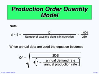
44. Production Order Quantity Model Q = Number of pieces per order p = Daily production rate H = Holding cost per unit per year d = Daily demand/usage rate D = Annual demand Q 2 = 2DS H[1 - (d/p)] Q* = 2DS H[1 - (d/p)] p Setup cost = (D/Q)S Holding cost = HQ[1 - (d/p)] 1 2 (D/Q)S = HQ[1 - (d/p)] 1 2

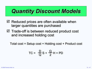
45. Production Order Quantity Example D = 1,000 units p = 8 units per day S = $10 d = 4 units per day H = $0.50 per unit per year Q* = 2DS H[1 - (d/p)] = 282.8 or 283 hubcaps Q* = = 80,000 2(1,000)(10) 0.50[1 - (4/8)]

46. Production Order Quantity Model When annual data are used the equation becomes Note: Q* = 2DS annual demand rate annual production rate H 1 – d = 4 = = D Number of days the plant is in operation 1,000 250

47. Quantity Discount Models Reduced prices are often available when larger quantities are purchased Trade-off is between reduced product cost and increased holding cost Total cost = Setup cost + Holding cost + Product cost TC = S + H + PD D Q Q 2

48. Quantity Discount Models Table 12.2 A typical quantity discount schedule Discount Number Discount Quantity Discount (%) Discount Price (P) 1 0 to 999 no discount $5.00 2 1,000 to 1,999 4 $4.80 3 2,000 and over 5 $4.75

49. Quantity Discount Models For each discount, calculate Q* If Q* for a discount doesn’t qualify, choose the smallest possible order size to get the discount Compute the total cost for each Q* or adjusted value from Step 2 Select the Q* that gives the lowest total cost Steps in analyzing a quantity discount

50. Quantity Discount Models Figure 12.7 1,000 2,000 Total cost $ 0 Order quantity Q* for discount 2 is below the allowable range at point a and must be adjusted upward to 1,000 units at point b a b 1st price break 2nd price break Total cost curve for discount 1 Total cost curve for discount 2 Total cost curve for discount 3

51. Quantity Discount Example Calculate Q* for every discount Q* = 2DS IP Q 1 * = = 700 cars/order 2(5,000)(49) (.2)(5.00) Q 2 * = = 714 cars/order 2(5,000)(49) (.2)(4.80) Q 3 * = = 718 cars/order 2(5,000)(49) (.2)(4.75)

52. Quantity Discount Example Calculate Q* for every discount Q* = 2DS IP Q 1 * = = 700 cars/order 2(5,000)(49) (.2)(5.00) Q 2 * = = 714 cars/order 2(5,000)(49) (.2)(4.80) Q 3 * = = 718 cars/order 2(5,000)(49) (.2)(4.75) 1,000 — adjusted 2,000 — adjusted

53. Quantity Discount Example Table 12.3 Choose the price and quantity that gives the lowest total cost Buy 1,000 units at $4.80 per unit Discount Number Unit Price Order Quantity Annual Product Cost Annual Ordering Cost Annual Holding Cost Total 1 $5.00 700 $25,000 $350 $350 $25,700 2 $4.80 1,000 $24,000 $245 $480 $24,725 3 $4.75 2,000 $23.750 $122.50 $950 $24,822.50

54. Probabilistic Models and Safety Stock Used when demand is not constant or certain Use safety stock to achieve a desired service level and avoid stockouts ROP = d x L + ss Annual stockout costs = the sum of the units short x the probability x the stockout cost/unit x the number of orders per year

55. Probabilistic Demand Figure 12.8 Safety stock 16.5 units ROP  Place order Inventory level Time 0 Minimum demand during lead time Maximum demand during lead time Mean demand during lead time Normal distribution probability of demand during lead time Expected demand during lead time (350 kits) ROP = 350 + safety stock of 16.5 = 366.5 Receive order Lead time

56. Probabilistic Demand Safety stock Probability of no stockout 95% of the time Mean demand 350 ROP = ? kits Quantity Number of standard deviations 0 z Risk of a stockout (5% of area of normal curve)

57. Probabilistic Demand Use prescribed service levels to set safety stock when the cost of stockouts cannot be determined ROP = demand during lead time + Z  dLT where Z = number of standard deviations  dLT = standard deviation of demand during lead time

58. Probabilistic Example Average demand =  = 350 kits Standard deviation of demand during lead time =  dLT = 10 kits 5% stockout policy (service level = 95%) Using Appendix I, for an area under the curve of 95%, the Z = 1.65 Safety stock = Z  dLT = 1.65(10) = 16.5 kits Reorder point = expected demand during lead time + safety stock = 350 kits + 16.5 kits of safety stock = 366.5 or 367 kits

59. Other Probabilistic Models When demand is variable and lead time is constant When lead time is variable and demand is constant When both demand and lead time are variable When data on demand during lead time is not available, there are other models available

60. Other Probabilistic Models Demand is variable and lead time is constant ROP = (average daily demand x lead time in days) + Z  dLT where  d = standard deviation of demand per day  dLT =  d lead time

61. Probabilistic Example Average daily demand (normally distributed) = 15 Standard deviation = 5 Lead time is constant at 2 days 90% service level desired Z for 90% = 1.28 From Appendix I Safety stock is about 9 iPods ROP = (15 units x 2 days) + Z  dlt = 30 + 1.28(5)( 2) = 30 + 9.02 = 39.02 ≈ 39

62. Other Probabilistic Models Lead time is variable and demand is constant ROP = (daily demand x average lead time in days) = Z x (daily demand) x  LT where  LT = standard deviation of lead time in days

63. Probabilistic Example Daily demand (constant) = 10 Average lead time = 6 days Standard deviation of lead time =  LT = 3 98% service level desired Z for 98% = 2.055 From Appendix I ROP = (10 units x 6 days) + 2.055(10 units)(3) = 60 + 61.65 = 121.65 Reorder point is about 122 cameras

64. Other Probabilistic Models Both demand and lead time are variable ROP = (average daily demand x average lead time) + Z  dLT where  d = standard deviation of demand per day  LT = standard deviation of lead time in days  dLT = (average lead time x  d 2 ) + (average daily demand) 2 x  LT 2

65. Probabilistic Example Average daily demand (normally distributed) = 150 Standard deviation =  d = 16 Average lead time 5 days (normally distributed) Standard deviation =  LT = 1 day 95% service level desired Z for 95% = 1.65 From Appendix I ROP = (150 packs x 5 days) + 1.65  dLT = (150 x 5) + 1.65 (5 days x 16 2 ) + (150 2 x 1 2 ) = 750 + 1.65(154) = 1,004 packs

66. Fixed-Period (P) Systems Orders placed at the end of a fixed period Inventory counted only at end of period Order brings inventory up to target level Only relevant costs are ordering and holding Lead times are known and constant Items are independent from one another

67. Fixed-Period (P) Systems Figure 12.9 On-hand inventory Time Q 1 Q 2 Target quantity (T) P Q 3 Q 4 P P

68. Fixed-Period (P) Example Order amount (Q) = Target (T) - On-hand inventory - Earlier orders not yet received + Back orders Q = 50 - 0 - 0 + 3 = 53 jackets 3 jackets are back ordered No jackets are in stock It is time to place an order Target value = 50

69. Fixed-Period Systems Inventory is only counted at each review period May be scheduled at convenient times Appropriate in routine situations May result in stockouts between periods May require increased safety stock