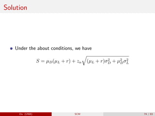
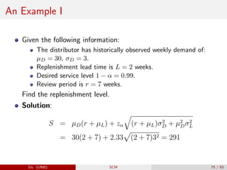
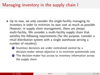
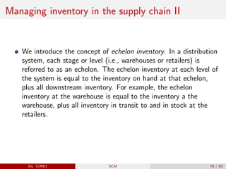
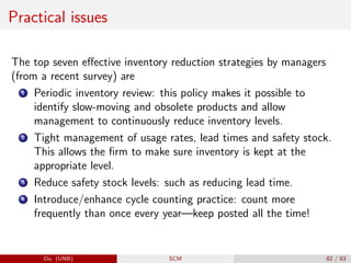
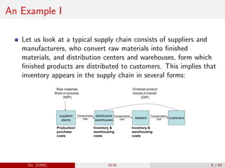
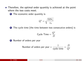
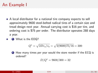
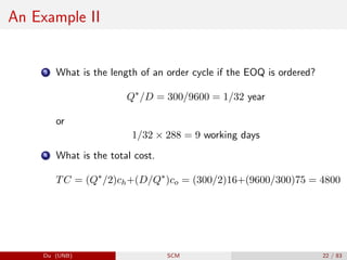
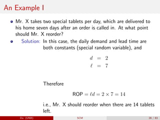
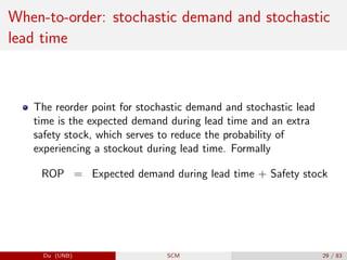
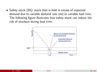
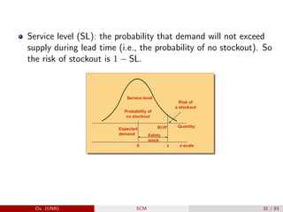
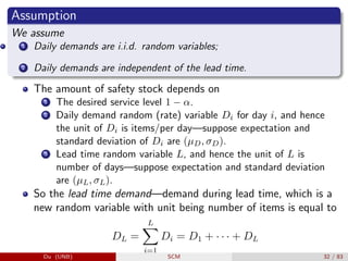
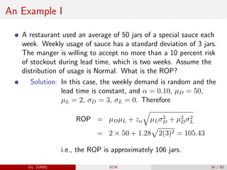
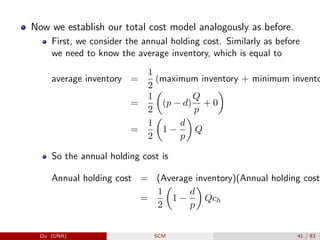
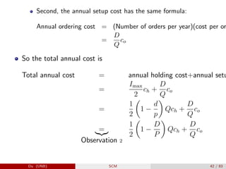
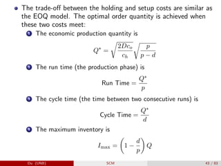
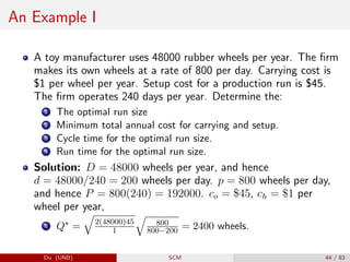
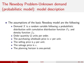
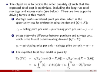
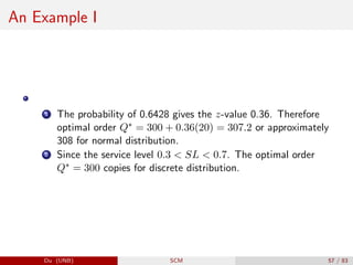
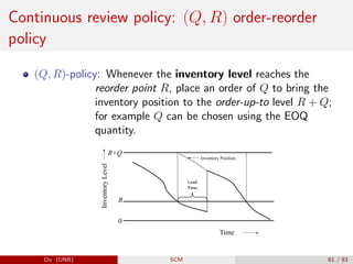
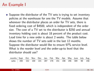
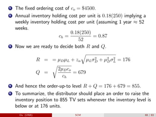
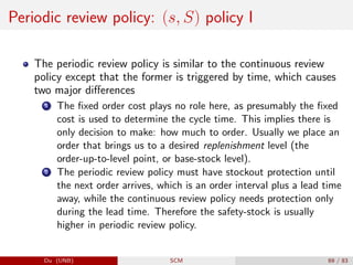
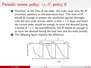
The document provides an overview of inventory management within the supply chain, detailing various inventory types, management objectives, and models such as Economic Order Quantity (EOQ) and Economic Production Quantity (EPQ). It emphasizes the importance of measuring inventory levels, safety stock, and reorder points to optimize service levels while minimizing costs. Additionally, it explores the decision-making process involved in determining how much and when to order inventory based on demand and lead time.

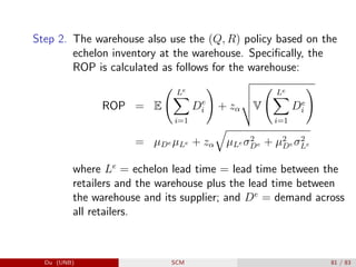
![Then, we use the compound random variable property to find
the expectation and variance of DL (note that here both Di’s
and L are random variable and we cannot apply the rule of
expectation and rule of variance directly):
E[DL] = E
L
P
i=1
Di
= µLµD
V[DL] = V
L
P
i=1
Di
= µLσ2
D + σ2
Lµ2
D
Assume DL follows a normal distribution, that is
DL ∼ N(E[DL],
p
V[DL]).
Then ROP should be chosen such that the probability of no
stockout is at least 1 − α, that is
P(DL ≤ ROP) ≥ 1 − α
A standard given-p-value-find-x-value calculation gives us the
desired ROP:
ROP = E[DL] + zα
p
V[DL] = µDµL + zα
q
µLσ2
D + µ2
Dσ2
L
Du (UNB) SCM 33 / 83](https://image.slidesharecdn.com/pptduinventorymanagement-240919234711-ef53f7ca/85/Supply-Chain-Management-Inventory-Management-33-320.jpg)
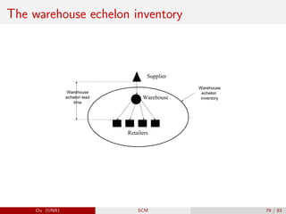
![A situation where we can decide s and Q I
The lead time L is a random variable.
Daily demand Di is random variable, i = 1, . . . , L.
The demand during lead time DL =
PL
i=1 Di follows a normal
distribution, whose expectation and variance can be calculated
similarly as before:
E[DL] = E
L
P
i=1
Di
= µLµD
V[DL] = V
L
P
i=1
Di
= µLσ2
D + σ2
Lµ2
D
There is an inventory holding cost of ch per unit per day.
There is a fixed order cost co per unit.
no backorders: when there is a stockout, the order is lost.
Du (UNB) SCM 63 / 83](https://image.slidesharecdn.com/pptduinventorymanagement-240919234711-ef53f7ca/85/Supply-Chain-Management-Inventory-Management-63-320.jpg)

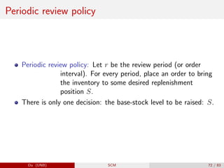
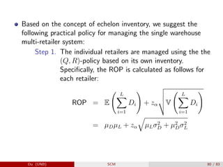
![A situation where we can decide S
Review period is r, a deterministic number.
The lead time L is a random variable.
Daily demand Di is random variable, i = 1, . . . , L.
The demand during lead time plus review period DL =
PL+r
i=1 Di
follows a normal distribution, whose expectation and variance
can be calculated similarly as before:
E[DL+r] = E
L+r
P
i=1
Di
= (r + µL)µD
V[DL+r] = V
L+r
P
i=1
Di
= (r + µL)σ2
D + σ2
Lµ2
D
no backorders: when there is a stockout, the order is lost.
There is a required service level of 1 − α. That is, the probability
of no-stockout during lead time is 1 − α
Du (UNB) SCM 73 / 83](https://image.slidesharecdn.com/pptduinventorymanagement-240919234711-ef53f7ca/85/Supply-Chain-Management-Inventory-Management-73-320.jpg)