Chapter 12:
Inventory Control Models
© 2007 Pearson Education
Inventory
• Any stored resource used to satisfy a
current or future need (raw materials,
work-in-process, finished goods, etc.)
• Represents as much as 50% of invested
capitol at some companies
• Excessive inventory levels are costly
• Insufficient inventory levels lead to
stockouts
Inventory Planning and Control
For maintaining the right balance between high
and low inventory to minimize cost
Main Uses of Inventory
1. The decoupling function
2. Storing resources
3. Irregular supply and demand
4. Quantity discounts
5. Avoiding stockouts and shortages
Inventory Control Decisions
Objective: Minimize total inventory cost
Decisions:
• How much to order?
• When to order?
Components of Total Cost
1. Cost of items
2. Cost of ordering
3. Cost of carrying or holding inventory
4. Cost of stockouts
5. Cost of safety stock (extra inventory held
to help avoid stockouts)
Economic Order Quantity (EOQ):
Determining How Much to Order
• One of the oldest and most well known
inventory control techniques
• Easy to use
• Based on a number of assumptions
Assumptions of the EOQ Model
1. Demand is known and constant
2. Lead time is known and constant
3. Receipt of inventory is instantaneous
4. Quantity discounts are not available
5. Variable costs are limited to: ordering
cost and carrying (or holding) cost
6. If orders are placed at the right time,
stockouts can be avoided
Inventory Level Over Time
Based on EOQ Assumptions
Minimizing EOQ Model Costs
• Only ordering and carrying costs need to
be minimized (all other costs are assumed
constant)
• As Q (order quantity) increases:
–Carry cost increases
–Ordering cost decreases (since the
number of orders per year decreases)
EOQ Model Total Cost
At optimal order quantity (Q*):
Carrying cost = Ordering cost
Finding the Optimal Order Quantity
Parameters:
Q* = Optimal order quantity (the EOQ)
D = Annual demand
Co = Ordering cost per order
Ch = Carrying (or holding) cost per unit per yr
P = Purchase cost per unit
Two Methods for Carrying Cost
Carry cost (Ch) can be expressed either:
1. As a fixed cost, such as
Ch = $0.50 per unit per year
2. As a percentage of the item’s purchase
cost (P)
Ch = I x P
I = a percentage of the purchase cost
EOQ Total Cost
Total ordering cost = (D/Q) x Co
Total carrying cost = (Q/2) x Ch
Total purchase cost = P x D
= Total cost
Note:
• (Q/2) is the average inventory level
• Purchase cost does not depend on Q
Finding Q*
Recall that at the optimal order quantity (Q*):
Carry cost = Ordering cost
(D/Q*) x Co = (Q*/2) x Ch
Rearranging to solve for Q*:
Q* = )/2( hCDCo
EOQ Example: Sumco Pump Co.
Buys pump housing from a manufacturer
and sells to retailers
D = 1000 pumps annually
Co = $10 per order
Ch = $0.50 per pump per year
P = $5
Q* = ?
Using ExcelModules for Inventory
• Worksheet for inventory models in
ExcelModules are color coded
– Input cells are yellow
– Output cells are green
• Select “Inventory Models” from the
ExcelModules menu, then select “EOQ”
Go to file 12-2.xls
Average Inventory Value
After Q* is found we can calculate the
average value of inventory on hand
Average inventory value = P x (Q*/2)
Calculating Ordering and
Carrying Costs for a Given Q
• Sometimes Co and Ch are difficult to
estimate
• We can use the EOQ formula to calculate
the value of Co or Ch that would make a
given Q optimal:
Co = Q2
x Ch/(2D)
Ch = 2DCo/Q2
Sensitivity of the EOQ Formula
• The EOQ formula assumes all inputs are
know with certainty
• In reality these values are often estimates
• Determining the effect of input value
changes on Q* is called sensitivity
analysis
Sensitivity Analysis for Sumco
• Suppose Co = $15 (instead of $10), which
is a 50% increase
• Assume all other values are unchanged
• The new Q* = 245 (instead of 200), which
is a 22.5% increase
• This shows the nonlinear nature of the
formula
Reorder Point:
Determining When to Order
• After Q* is determined, the second
decision is when to order
• Orders must usually be placed before
inventory reaches 0 due to order lead time
• Lead time is the time from placing the
order until it is received
• The reorder point (ROP) depends on the
lead time (L)
Reorder Point (ROP)
ROP = d x L
Sumco Example Revisited
• Assume lead time, L = 3 business days
• Assume 250 business days per year
• Then daily demand,
d = 1000 pumps/250 days = 4 pumps per day
ROP = (4 pumps per day) x (3 days)
= 12 pumps
Go to file 12-3.xls
Economic Production Quantity:
Determining How Much to Produce
• The EOQ model assumes inventory
arrives instantaneously
• In many cases inventory arrives gradually
• The economic production quantity
(EPQ) model assumes inventory is being
produced at a rate of p units per day
• There is a setup cost each time
production begins
Inventory Control With Production
Determining Lot Size or EPQ
Parameters
Q* = Optimal production quantity (or EPQ)
Cs = Setup cost
D = annual demand
d = daily demand rate
p = daily production rate
Average Inventory Level
• We will need the average inventory level
for finding carrying cost
• Average inventory level is ½ the maximum
Max inventory = Q x (1- d/p)
Ave inventory = ½ Q x (1- d/p)
Total Cost
Setup cost = (D/Q) x Cs
Carrying cost = [½ Q x (1- d/p)] x
Ch
Production cost = P x D
= Total cost
As in the EOQ model:
• The production cost does not depend on Q
• The function is nonlinear
Finding Q*
• As in the EOQ model, at the optimal quantity
Q* we should have:
Setup cost = Carrying cost
(D/Q*) x Cs = [½ Q* x (1- d/p)] x Ch
Rearranging to solve for Q*:
Q* = )]/1(/[2( pdCDC hs −
EPQ for Brown Manufacturing
Produces mini refrigerators (has 167
business days per year)
D = 10,000 units annually
d = 1000 / 167 = ~60 units per day
p = 80 units per day (when producing)
Ch = $0.50 per unit per year
Cs = $100 per setup
P = $5 to produce each unit
Go to file 12-4.xls
Length of the Production Cycle
• The production cycle will last until Q* units
have been produced
• Producing at a rate of p units per day
means that it will last (Q*/p) days
• For Brown this is:
Q* = 4000 units
p = 80 units per day
4000 / 80 = 50 days
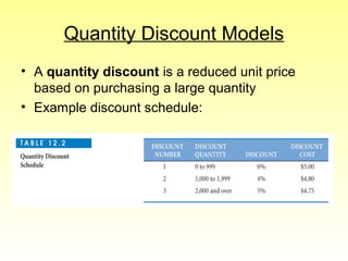
Quantity Discount Models
• A quantity discount is a reduced unit price
based on purchasing a large quantity
• Example discount schedule:
Four Steps to Analyze
Quantity Discount Models
1. Calculate Q* for each discount price
2. If Q* is too small to qualify for that price,
adjust Q* upward
3. Calculate total cost for each Q*
4. Select the Q* with the lowest total cost
Brass Department Store Example
Sells toy cars
D = 5000 cars annually
Co = $49 per order
Ch = $0.20 per car per year
Quantity Discount Schedule
go to file 12-5.xls
Use of Safety Stock
• Safety stock (SS) is extra inventory held
to help prevent stockouts
• Frequently demand is subject to random
variability (uncertainty)
• If demand is unusually high during lead
time, a stockout will occur if there is no
safety stock
Use of Safety Stock
Determining Safety Stock Level
Need to know:
• Probability of demand during lead time
(DDLT)
• Cost of a stockout (includes all costs
directly or indirectly associated, such as
cost of a lost sale and future lost sales)
ABCO Safety Stock Example
• ROP = 50 units (from previous EOQ)
• Place 6 orders per year
• Stockout cost per unit = $40
• Ch = $5 per unit per year
• DDLT has a discrete distribution
Analyzing the Alternatives
• With uncertain DDLT this becomes a
“decision making under risk” problem
• Each of the five possible values of DDLT
represents a decision alternative for ROP
• Need to determine the economic payoff
for each combination of decision
alternative (ROP) and outcome (DDLT)
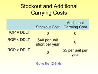
Stockout and Additional
Carrying Costs
Stockout Cost
Additional
Carrying Cost
ROP = DDLT 0 0
ROP < DDLT $40 per unit
short per year
0
ROP > DDLT
0
$5 per unit per
year
Go to file 12-6.xls
Safety Stock With
Unknown Stockout Costs
• Determining stockout costs may be difficult
or impossible
• Customer dissatisfaction and possible
future lost sales are difficult to estimate
• Can use service level instead
Service level = 1 – probability of a stockout
Hinsdale Co. Example
• DDLT follows a normal distribution
(μ = 350, σ = 10)
• They want a 95% service level (i.e. 5%
probability of a stockout)
SS = ?
Safety Stock and the Normal
Distribution
Calculating SS
From the standard Normal Table,
Z = 1.645 = X – 350 so X= 366.45
10
and, SS = 16.45 (which could be rounded
to17)
Hinsdale’s Carrying Cost
• Assume Hinsdale has a carrying cost of
$1 per unit per year
• We can calculate the SS and its carrying
cost for various service levels
Cost of Different Service Levels
Carrying Cost Versus Service Level
Go to file 12-7.xls
ABC Analysis
• Recognizes that some inventory items are
more important than others
• A group items are considered critical
(often about 70% of dollar value and 10%
of items)
• B group items are important but not critical
(often about 20% of dollar value and 20%
of items)
• C group items are not as important (often
about 10% of dollar value and 70% of
items)
Silicon Chips Inc. Example
• Maker of super fast DRAM chips
• Has 10 inventory items
• Wants to classify them into A, B, and C
groups
• Calculate dollar value of each item and
rank items
Go to file 12-8.xls
Inventory Items for Silicon Chips

INVENTORY CONTROL

  • 1.
    Chapter 12: Inventory ControlModels © 2007 Pearson Education
  • 2.
    Inventory • Any storedresource used to satisfy a current or future need (raw materials, work-in-process, finished goods, etc.) • Represents as much as 50% of invested capitol at some companies • Excessive inventory levels are costly • Insufficient inventory levels lead to stockouts
  • 3.
    Inventory Planning andControl For maintaining the right balance between high and low inventory to minimize cost
  • 4.
    Main Uses ofInventory 1. The decoupling function 2. Storing resources 3. Irregular supply and demand 4. Quantity discounts 5. Avoiding stockouts and shortages
  • 5.
    Inventory Control Decisions Objective:Minimize total inventory cost Decisions: • How much to order? • When to order?
  • 6.
    Components of TotalCost 1. Cost of items 2. Cost of ordering 3. Cost of carrying or holding inventory 4. Cost of stockouts 5. Cost of safety stock (extra inventory held to help avoid stockouts)
  • 7.
    Economic Order Quantity(EOQ): Determining How Much to Order • One of the oldest and most well known inventory control techniques • Easy to use • Based on a number of assumptions
  • 8.
    Assumptions of theEOQ Model 1. Demand is known and constant 2. Lead time is known and constant 3. Receipt of inventory is instantaneous 4. Quantity discounts are not available 5. Variable costs are limited to: ordering cost and carrying (or holding) cost 6. If orders are placed at the right time, stockouts can be avoided
  • 9.
    Inventory Level OverTime Based on EOQ Assumptions
  • 10.
    Minimizing EOQ ModelCosts • Only ordering and carrying costs need to be minimized (all other costs are assumed constant) • As Q (order quantity) increases: –Carry cost increases –Ordering cost decreases (since the number of orders per year decreases)
  • 11.
    EOQ Model TotalCost At optimal order quantity (Q*): Carrying cost = Ordering cost
  • 12.
    Finding the OptimalOrder Quantity Parameters: Q* = Optimal order quantity (the EOQ) D = Annual demand Co = Ordering cost per order Ch = Carrying (or holding) cost per unit per yr P = Purchase cost per unit
  • 13.
    Two Methods forCarrying Cost Carry cost (Ch) can be expressed either: 1. As a fixed cost, such as Ch = $0.50 per unit per year 2. As a percentage of the item’s purchase cost (P) Ch = I x P I = a percentage of the purchase cost
  • 14.
    EOQ Total Cost Totalordering cost = (D/Q) x Co Total carrying cost = (Q/2) x Ch Total purchase cost = P x D = Total cost Note: • (Q/2) is the average inventory level • Purchase cost does not depend on Q
  • 15.
    Finding Q* Recall thatat the optimal order quantity (Q*): Carry cost = Ordering cost (D/Q*) x Co = (Q*/2) x Ch Rearranging to solve for Q*: Q* = )/2( hCDCo
  • 16.
    EOQ Example: SumcoPump Co. Buys pump housing from a manufacturer and sells to retailers D = 1000 pumps annually Co = $10 per order Ch = $0.50 per pump per year P = $5 Q* = ?
  • 17.
    Using ExcelModules forInventory • Worksheet for inventory models in ExcelModules are color coded – Input cells are yellow – Output cells are green • Select “Inventory Models” from the ExcelModules menu, then select “EOQ” Go to file 12-2.xls
  • 18.
    Average Inventory Value AfterQ* is found we can calculate the average value of inventory on hand Average inventory value = P x (Q*/2)
  • 19.
    Calculating Ordering and CarryingCosts for a Given Q • Sometimes Co and Ch are difficult to estimate • We can use the EOQ formula to calculate the value of Co or Ch that would make a given Q optimal: Co = Q2 x Ch/(2D) Ch = 2DCo/Q2
  • 20.
    Sensitivity of theEOQ Formula • The EOQ formula assumes all inputs are know with certainty • In reality these values are often estimates • Determining the effect of input value changes on Q* is called sensitivity analysis
  • 21.
    Sensitivity Analysis forSumco • Suppose Co = $15 (instead of $10), which is a 50% increase • Assume all other values are unchanged • The new Q* = 245 (instead of 200), which is a 22.5% increase • This shows the nonlinear nature of the formula
  • 22.
    Reorder Point: Determining Whento Order • After Q* is determined, the second decision is when to order • Orders must usually be placed before inventory reaches 0 due to order lead time • Lead time is the time from placing the order until it is received • The reorder point (ROP) depends on the lead time (L)
  • 23.
  • 24.
    Sumco Example Revisited •Assume lead time, L = 3 business days • Assume 250 business days per year • Then daily demand, d = 1000 pumps/250 days = 4 pumps per day ROP = (4 pumps per day) x (3 days) = 12 pumps Go to file 12-3.xls
  • 25.
    Economic Production Quantity: DeterminingHow Much to Produce • The EOQ model assumes inventory arrives instantaneously • In many cases inventory arrives gradually • The economic production quantity (EPQ) model assumes inventory is being produced at a rate of p units per day • There is a setup cost each time production begins
  • 26.
  • 27.
    Determining Lot Sizeor EPQ Parameters Q* = Optimal production quantity (or EPQ) Cs = Setup cost D = annual demand d = daily demand rate p = daily production rate
  • 28.
    Average Inventory Level •We will need the average inventory level for finding carrying cost • Average inventory level is ½ the maximum Max inventory = Q x (1- d/p) Ave inventory = ½ Q x (1- d/p)
  • 29.
    Total Cost Setup cost= (D/Q) x Cs Carrying cost = [½ Q x (1- d/p)] x Ch Production cost = P x D = Total cost As in the EOQ model: • The production cost does not depend on Q • The function is nonlinear
  • 30.
    Finding Q* • Asin the EOQ model, at the optimal quantity Q* we should have: Setup cost = Carrying cost (D/Q*) x Cs = [½ Q* x (1- d/p)] x Ch Rearranging to solve for Q*: Q* = )]/1(/[2( pdCDC hs −
  • 31.
    EPQ for BrownManufacturing Produces mini refrigerators (has 167 business days per year) D = 10,000 units annually d = 1000 / 167 = ~60 units per day p = 80 units per day (when producing) Ch = $0.50 per unit per year Cs = $100 per setup P = $5 to produce each unit Go to file 12-4.xls
  • 32.
    Length of theProduction Cycle • The production cycle will last until Q* units have been produced • Producing at a rate of p units per day means that it will last (Q*/p) days • For Brown this is: Q* = 4000 units p = 80 units per day 4000 / 80 = 50 days
  • 33.
    Quantity Discount Models •A quantity discount is a reduced unit price based on purchasing a large quantity • Example discount schedule:
  • 34.
    Four Steps toAnalyze Quantity Discount Models 1. Calculate Q* for each discount price 2. If Q* is too small to qualify for that price, adjust Q* upward 3. Calculate total cost for each Q* 4. Select the Q* with the lowest total cost
  • 35.
    Brass Department StoreExample Sells toy cars D = 5000 cars annually Co = $49 per order Ch = $0.20 per car per year Quantity Discount Schedule go to file 12-5.xls
  • 36.
    Use of SafetyStock • Safety stock (SS) is extra inventory held to help prevent stockouts • Frequently demand is subject to random variability (uncertainty) • If demand is unusually high during lead time, a stockout will occur if there is no safety stock
  • 37.
  • 38.
    Determining Safety StockLevel Need to know: • Probability of demand during lead time (DDLT) • Cost of a stockout (includes all costs directly or indirectly associated, such as cost of a lost sale and future lost sales)
  • 39.
    ABCO Safety StockExample • ROP = 50 units (from previous EOQ) • Place 6 orders per year • Stockout cost per unit = $40 • Ch = $5 per unit per year • DDLT has a discrete distribution
  • 40.
    Analyzing the Alternatives •With uncertain DDLT this becomes a “decision making under risk” problem • Each of the five possible values of DDLT represents a decision alternative for ROP • Need to determine the economic payoff for each combination of decision alternative (ROP) and outcome (DDLT)
  • 41.
    Stockout and Additional CarryingCosts Stockout Cost Additional Carrying Cost ROP = DDLT 0 0 ROP < DDLT $40 per unit short per year 0 ROP > DDLT 0 $5 per unit per year Go to file 12-6.xls
  • 42.
    Safety Stock With UnknownStockout Costs • Determining stockout costs may be difficult or impossible • Customer dissatisfaction and possible future lost sales are difficult to estimate • Can use service level instead Service level = 1 – probability of a stockout
  • 43.
    Hinsdale Co. Example •DDLT follows a normal distribution (μ = 350, σ = 10) • They want a 95% service level (i.e. 5% probability of a stockout) SS = ?
  • 44.
    Safety Stock andthe Normal Distribution
  • 45.
    Calculating SS From thestandard Normal Table, Z = 1.645 = X – 350 so X= 366.45 10 and, SS = 16.45 (which could be rounded to17)
  • 46.
    Hinsdale’s Carrying Cost •Assume Hinsdale has a carrying cost of $1 per unit per year • We can calculate the SS and its carrying cost for various service levels
  • 47.
    Cost of DifferentService Levels
  • 48.
    Carrying Cost VersusService Level Go to file 12-7.xls
  • 49.
    ABC Analysis • Recognizesthat some inventory items are more important than others • A group items are considered critical (often about 70% of dollar value and 10% of items) • B group items are important but not critical (often about 20% of dollar value and 20% of items) • C group items are not as important (often about 10% of dollar value and 70% of items)
  • 50.
    Silicon Chips Inc.Example • Maker of super fast DRAM chips • Has 10 inventory items • Wants to classify them into A, B, and C groups • Calculate dollar value of each item and rank items
  • 51.
    Go to file12-8.xls Inventory Items for Silicon Chips