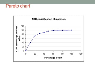
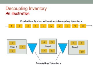
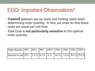
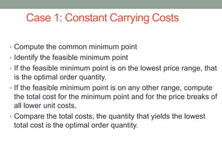
This document provides an overview of inventory management concepts. It discusses the meaning and types of inventory, related costs like ordering, carrying, and shortage costs. It introduces the basic Economic Order Quantity (EOQ) model, which aims to minimize total inventory costs by balancing ordering and carrying costs. The EOQ model formulas and assumptions are explained. It is noted that total costs are not very sensitive around the optimal order quantity. The document also discusses decoupling inventory, quantity discounts, and ABC classification of inventory items.

1. INVENTORY MANAGEMENT (I)
Dr. Debadyuti Das
Professor
FMS, DU
das_debadyuti@rediffmail.com

2. Broad outline
• Meaning of inventory in the context of Operations
& Supply Chain
• Inventory types
• Inventory-related costs
• Basic EOQ model
• Selective Inventory Control

3. Inventory: An overview
• Vital element of any organization which enables it
- to run its operation in an uninterrupted manner and
- to provide a satisfactory level of service to its customers.
• The issue is – how much inventory should an organization
keep – too much or too little?
• Trade-off between providing good customer service
versus achieving operating efficiency.
• Performance measures of inventory management:
inventory turnover ratio.
• Generally higher the ratio, better is the performance.
• Desirable number of turns depends on the type of industry
and the amount of profit margins.
• High-end retailers have a low turnover rate while
supermarkets have a fairly high turnover rate.

4. Inventory types
• On the basis of physical characteristics (or accounting
classification), inventory is divided into three main types:
- Raw materials and purchased parts
- Work-in-process (WIP) goods
- Finished goods
• On the basis of functional classification
- Cycle inventory
- Safety inventory
- Pipeline inventory
- Anticipation inventory
- Decoupling inventory

5. Decoupling Inventory
An illustration
1 2 3 4 5 6 7 8 9 10
1
2
3
4 5
6
7
8 9
10
Stage 2
Stage 1 Stage 3
Decoupling Inventory
Production System without any decoupling inventory

6. Quantity
Time
Safety stock
Cyclic
Stock
Pipeline stock
L
Cyclic, Pipeline and Safety Stocks
A graphical illustration
Cyclic inventory, pipeline inventory and safety stocks are critically linked to
“how much” and “when” decisions in inventory planning

7. Inventory related costs
• Ordering costs:
Costs associated with the preparation of purchase order,
getting the necessary approval for placing the purchase order, actual
placing of the order and follow-up of the same.
• Carrying costs:
Costs incurred in connection with the physical storage of items.
• Shortage costs:
Costs incurred by the firm when demand exceeds supply of
inventory on hand. There are two types of shortage costs:
(i) lost sales cost and
(ii) backorder cost.

8. Basic EOQ model
• Assumptions of the basic EOQ model:
- Only one product is involved
- Annual demand requirements are known
- Demand is even throughout the year
- Lead time does not vary
- Each order is received in a single delivery
- There are no quantity discounts

9. The Inventory Cycle
Profile of Inventory Level Over Time
Quantity
on hand
Q
Receive
order
Place
order
Receive
order
Place
order
Receive
order
Lead time
Reorder
point
Usage
rate
Time

10. Basic EOQ model
Notations:
• D: Annual demand
• A: Setup or Order Cost
• C: Cost per unit
• h: Holding cost per year as a percentage of unit product cost
• H: Inventory carrying costs per unit per year = h*C
• Q: Lot Size
• T: Reorder interval
• Number of orders per year = D/Q
• Annual material cost = C*D
• Annual order cost = (D/Q)*A
• Annual holding cost = (Q/2)*H
• Total annual variable cost (TC) = (D/Q)*A + (Q/2)*H

11. Cost Minimization Goal
Order Quantity
(Q)
The Total-Cost Curve is U-Shaped
Ordering Costs
QO
Annual
Cost
(optimal order quantity)
A
Q
D
H
Q
TC 

2

12. Deriving the EOQ
Using calculus, we take the derivative of the total cost
function and set the derivative (slope) equal to zero and
solve for Q.
Q =
2DS
H
=
2(Annual Demand )(Order or Setup Cost )
Annual Holding Cost
OPT

13. Basic EOQ model
• The total cost curve reaches its minimum where the
carrying and ordering costs are equal, i.e.
Q/2 *(H) = (D/Q)*A
i.e.
Key insights:
• Total cost curve is relatively flat in the vicinity of EOQ. This indicates
that the total cost is not particularly sensitive to the optimal order
quantity.
• In deciding the optimal lot size, the tradeoff is between order (set-up)
cost and holding cost.
• If demand increases by a factor of k, it is optimal to increase batch
size by a factor of Sqrt k.
• If lot size is to be reduced, one has to reduce fixed order cost.

14. EOQ: Important Observations*
• Tradeoff between set-up costs and holding costs when
determining order quantity. In fact, we order so that these
costs are equal per unit time.
• Total Cost is not particularly sensitive to the optimal
order quantity.
Order Quantity 50% 80% 90% 100% 110% 120% 150% 200%
Increase in cost 25% 2.5 % 0.5 % 0 % 0.4 % 1.6 % 8.0 % 25.0 %

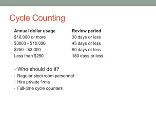
15. Example (1)
Demand, D = 12,000 computers per year
d = 1000 computers/month
Unit cost, C = $500
Holding cost fraction, h = 0.2
Fixed ordering cost, A = $4,000/order
Q* = Sqrt[(2)(12000)(4000)/(0.2)(500)] = 980 computers
Cycle inventory = Q/2 = 490
Flow time = (Q/2d) = 980/(2)(1000) = 0.49 month
No. of orders per year = (D/Q) = 12,000/980 = 12.24
Reorder interval, T = (Q/d) = 0.98 month

16. Example 1(continued)
Annual ordering and holding cost =
= (12000/980)(4000) + (980/2)(0.2)(500) = $97,980
Suppose lot size is reduced to Q = 200, which would reduce
flow time:
Annual ordering and holding cost =
= (12000/200)(4000) + (200/2)(0.2)(500) = $250,000
To make it economically feasible to reduce lot size, the fixed
cost associated with each lot would have to be reduced

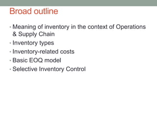
17. Example 2
If desired lot size Q* = 200 units, what would A have
to be?
D = 12000 units
C = $500
h = 0.2
Use EOQ equation and solve for A:
A = [hC(Q*)2]/2D
= [(0.2)(500)(200)2]/(2)(12000)
= $166.67
To reduce optimal lot size by a factor of k, the fixed order cost
must be reduced by a factor of k2

18. Key Points from EOQ Model
• In deciding the optimal lot size, the tradeoff is between
setup (order) cost and holding cost.
• If demand increases by a factor of k, it is optimal to
increase batch size by a factor of Sqrt k. No of orders
placed per year should increase by a factor of Sqrt k. Flow
time attributed to Cycle inventory should decrease by a
factor of Sqrt k.
• If lot size is to be reduced, one has to reduce fixed order
cost. To reduce lot size by a factor of 2, order cost has to be
reduced by a factor of 4.

19. Economic Production Quantity (EPQ)
• Production done in batches or lots
• Capacity to produce a part exceeds the part’s usage or
demand rate
• Assumptions of EPQ are similar to EOQ except orders
are received incrementally during production

20. Economic Production Quantity
Assumptions
• Only one item is involved
• Annual demand is known
• Usage rate is constant
• Usage occurs continually
• Production rate is constant
• Lead time does not vary
• No quantity discounts

21. Economic Run Size
Q
DS
H
p
p u
0
2



22. Total Costs with Purchasing Cost
Annual
carrying
cost
Purchasing
cost
TC = +
Q
2
H
D
Q
S
TC = +
+
Annual
ordering
cost
PD
+

23. Total Costs with PD
Cost
EOQ
TC with PD
TC without PD
PD
0 Quantity
Adding Purchasing cost
doesn’t change EOQ

24. All unit Quantity Discount Model
• Pricing schedule has specified quantity break points q0,
q1, …, qr, where q0 = 0
• If an order is placed that is at least as large as qi but
smaller than qi+1, then each unit has an average unit cost
of Ci
• The unit cost generally decreases as the quantity
increases, i.e., C0>C1>…>Cr
• The objective for the company (a retailer in our example)
is to decide on a lot size that will minimize the sum of
material, order, and holding costs

25. Case 1: Quantity Discount Model: Total Cost with
Constant Carrying Costs
OC
EOQ Quantity
Total
Cost
TCa
TCc
TCb
Decreasing
Price
CC a,b,c

26. Case 1: Constant Carrying Costs
• Compute the common minimum point
• Identify the feasible minimum point
• If the feasible minimum point is on the lowest price range, that
is the optimal order quantity.
• If the feasible minimum point is on any other range, compute
the total cost for the minimum point and for the price breaks of
all lower unit costs.
• Compare the total costs, the quantity that yields the lowest
total cost is the optimal order quantity.

27. Case 2: Quantity Discount Model: Total Cost with
Carrying Costs expressed as % of unit price
OC
EOQ Quantity
Total
Cost
TCa
TCc
TCb
Decreasing
Price
CCc
CCa
CCb

28. Case 2: Carrying Costs expressed as % of unit price
Step 1: Calculate the EOQ for the lowest price. If it is
feasible (i.e., this order quantity is in the range for that
price), then stop. This is the optimal lot size. Calculate TC
for this lot size.
Step 2: If the EOQ is not feasible, calculate the EOQ for the
next lowest price. If it is feasible, stop and calculate the TC
for that quantity.
Step 3: Calculate the TC corresponding to the lowest price
and the smallest quantity necessary to obtain the lowest
price.
Step 4: Compare the TC for Steps 2 and 3. Choose the
quantity corresponding to the lowest TC.
Step 5: If the EOQ in Step 3 is not feasible, repeat Steps 2,
3, and 4 until a feasible EOQ is found.

29. All-Unit Quantity Discounts: Example
Cost/Unit
$3
$2.96
$2.92
Order Quantity
5,000 10,000
Order Quantity
5,000 10,000
Total Material Cost

30. All-Unit Quantity Discount: Example
Order quantity Unit Price
0-5000 $3.00
5001-10000 $2.96
Over 10000 $2.92
q0 = 0, q1 = 5000, q2 = 10000
C0 = $3.00, C1 = $2.96, C2 = $2.92
D = 120000 units/year, S = $100/lot, h = 0.2

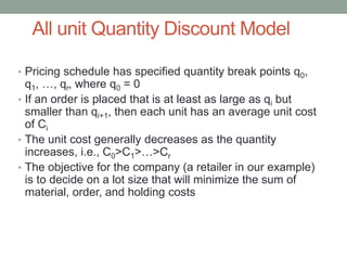
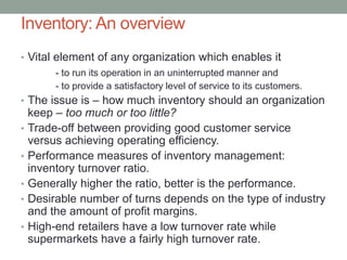
31. All-Unit Quantity Discount: Example
Step 1: Calculate Q2* = Sqrt[(2DS)/hC2]
= Sqrt[(2)(120000)(100)/(0.2)(2.92)] = 6410
Not feasible (6410 < 10001)
Calculate TC2 using C2 = $2.92 and q2 = 10001
TC2 =
(120000/10001)(100)+(10001/2)(0.2)(2.92)+(120000)(2.92)
= $354,520

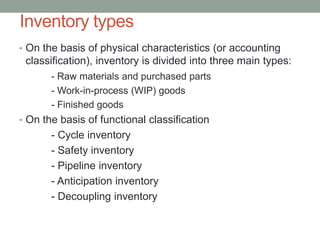
32. All-Unit Quantity Discount: Example
Step 2: Calculate Q1* = Sqrt[(2DS)/hC1]
=Sqrt[(2)(120000)(100)/(0.2)(2.96)] = 6367
Feasible (5000<6367<10000)  Stop
TC1 = (120000/6367)(100)+(6367/2)(0.2)(2.96)+
(120000)(2.96) = $358,969
TC2 < TC1  The optimal order quantity Q* is q2 = 10001

33. ABC Classification
• Items are classified into A, B and C category based
on the annual consumption value of items.
• ‘A’ category items: High value items and constitute
roughly 10% of the whole items but account for
approx. 70% of the total annual consumption value.
• ‘B’ category items: Medium value items and account
for approx. 20% of the whole items and contribute
towards 20% of the annual consumption value.
• ‘C’ category items: Low value items and constitute
roughly 70% of the items and account for only 10% of
the annual consumption value.

34. ABC classification

35. Pareto chart
ABC classification of materials
0
20
40
60
80
100
120
0 20 40 60 80 100 120
Percentage of item
Cum
percentage
of
rupee
value

36. VED classification
• Items are segregated on the basis of criticality of the items
specified by the end users.
• ‘V’ indicates vital items without which the entire
functioning of the plant or the machine gets severely
affected.
• ‘E’ indicates essential items required by the end users.
• ‘D’ denotes desirable items from the point of view of the
end users.
• This classification is quite popular in maintenance
management.

37. FSN classification
• Items are classified based on the volume of consumption.
• ‘F’ indicates fast moving items
• ‘S’ indicates slow moving and
• ‘N’ indicates non-moving items.
• Fast moving items generally kept in all decentralized
stores.
• Slow moving items generally stocked in a centralized
store.
• Non-moving items need to be disposed off gradually.

38. SDE classification
• Items are classified based on their availability in the market.
• ‘S’ means ‘scarce to obtain’, which further implies that the
items are probably available in international market.
• D’ implies ‘difficult to obtain’, which indicates that the items
are probably available in the national market.
• E’ indicates ‘easy to obtain’, which implies that the items
are probably available in local markets.
• Helps in developing suitable sourcing strategies for different
category of items.

39. Combination of ABC & VED classification
• Exercise control on high value and highly critical (vital)
items

40. Combination of ABC, VED & SDE
classification
• Exercise control on high value, vital and scarce to obtain
items.

41. Cycle Counting
• The purpose cycle counting is to reduce discrepancies
between the amounts indicated by inventory records and
actual quantities of inventory on hand.
• A physical inventory-taking technique in which inventory is
counted on a frequent basis rather than once or twice a
year.
• Every organization must have agreement within some
specified range between what the inventory record says is
in inventory and what actually is in inventory.
• There are many reasons why the records and the physical
inventory might not match.

42. Cycle Counting
• The key questions concerning cycle counting are:
How much accuracy is needed?
• A items: ± 0.2 percent
• B items: ± 1 percent
• C items: ± 5 percent
When should cycle counting be performed?
• When the record shows a low/zero balance on hand
• When record shows a positive balance but there has been a
backorder
• After some specified level of activity
• To signal a review based on the importance of the item

43. Cycle Counting
Annual dollar usage Review period
$10,000 or more 30 days or less
$3000 - $10,000 45 days or less
$250 - $3,000 90 days or less
Less than $250 180 days or less
Who should do it?
• Regular stockroom personnel
• Hire private firms
• Full-time cycle counters