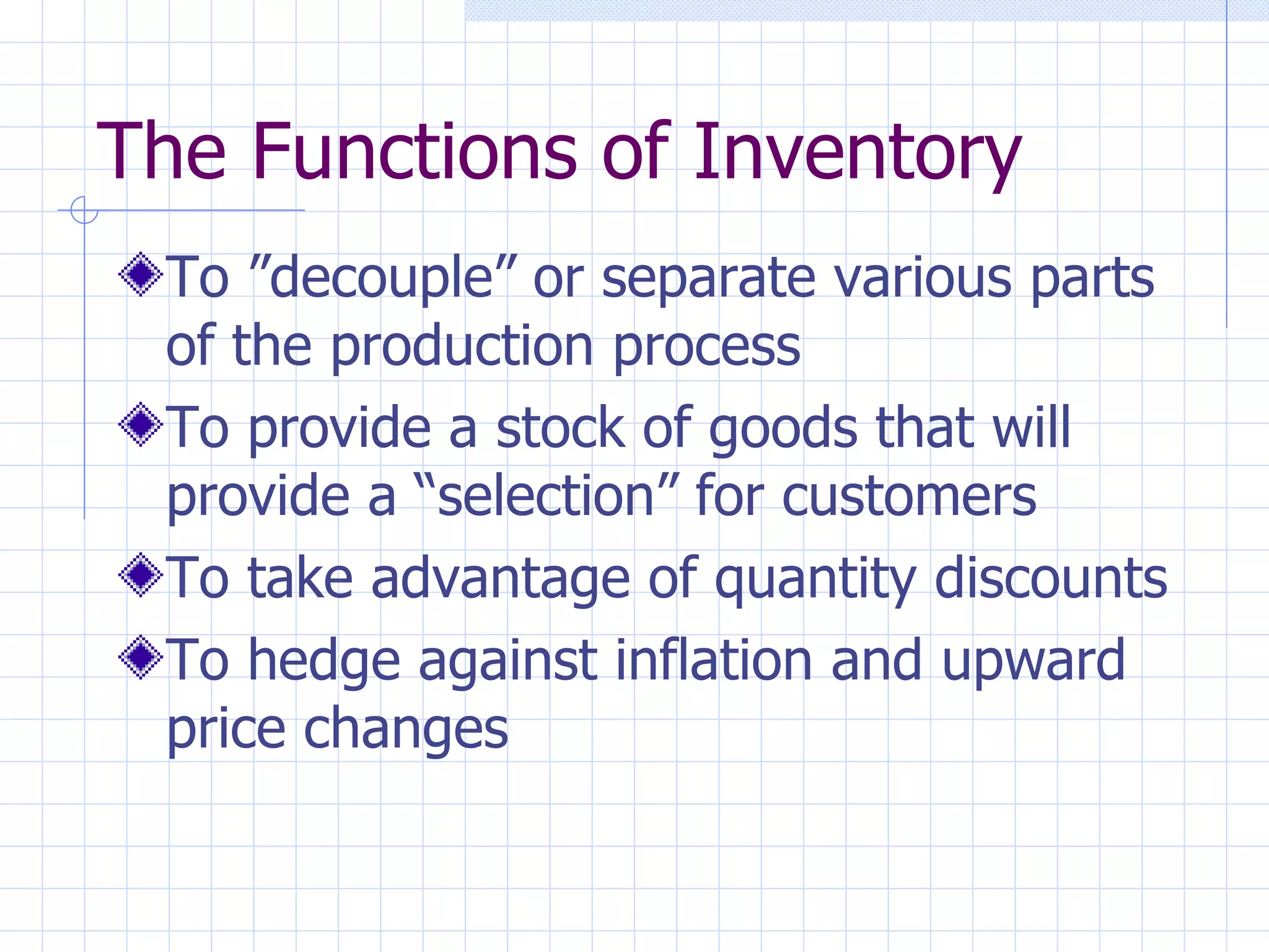
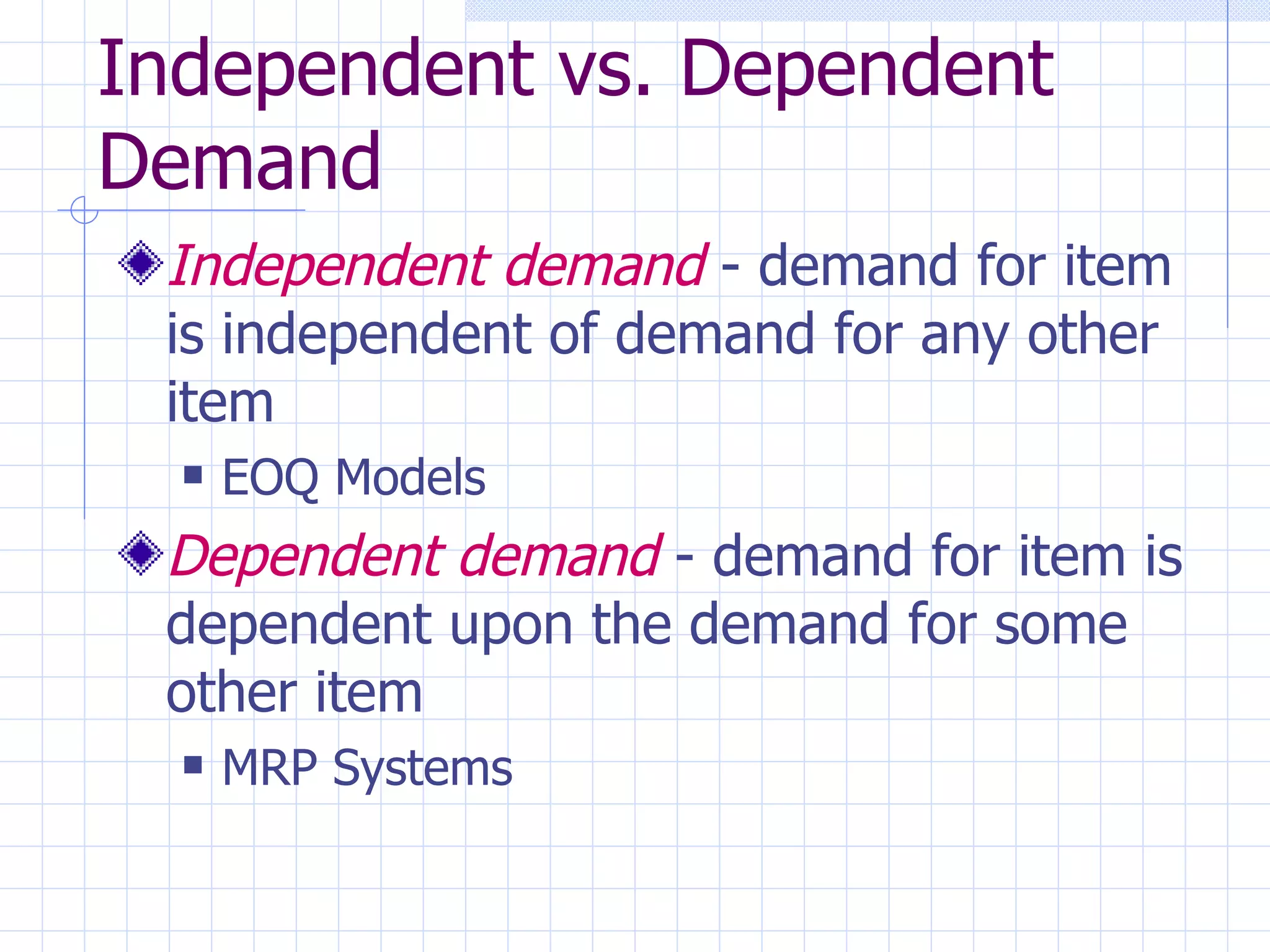
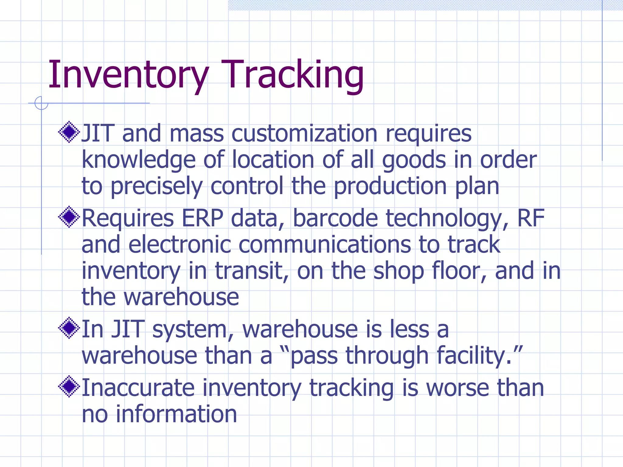
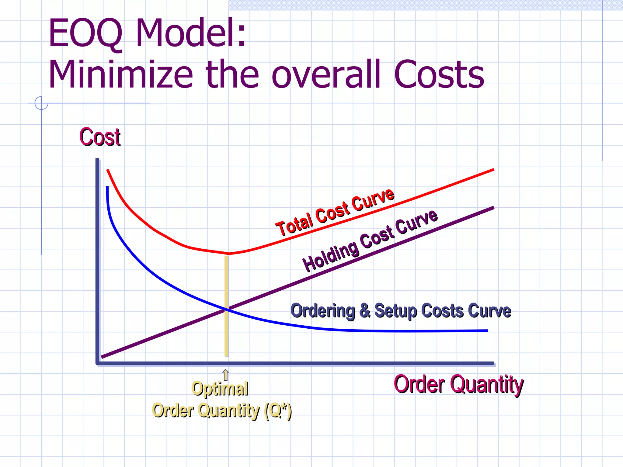
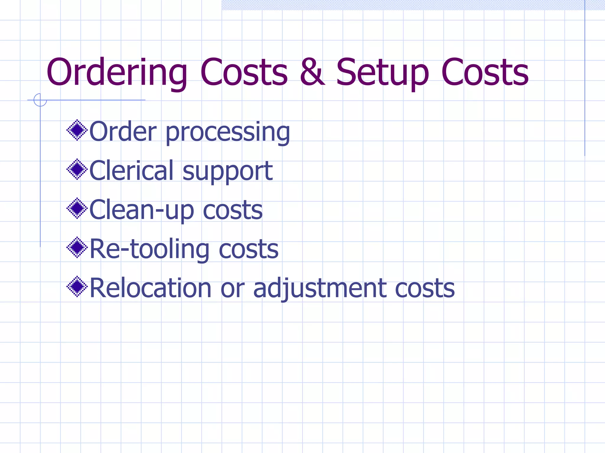
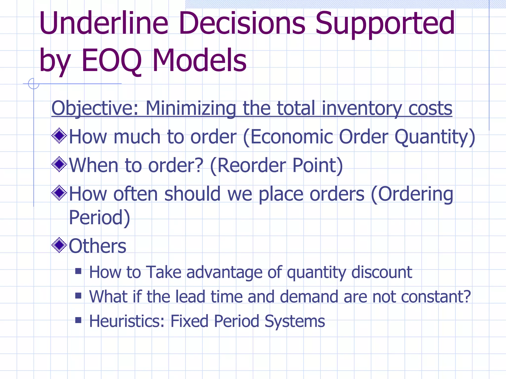
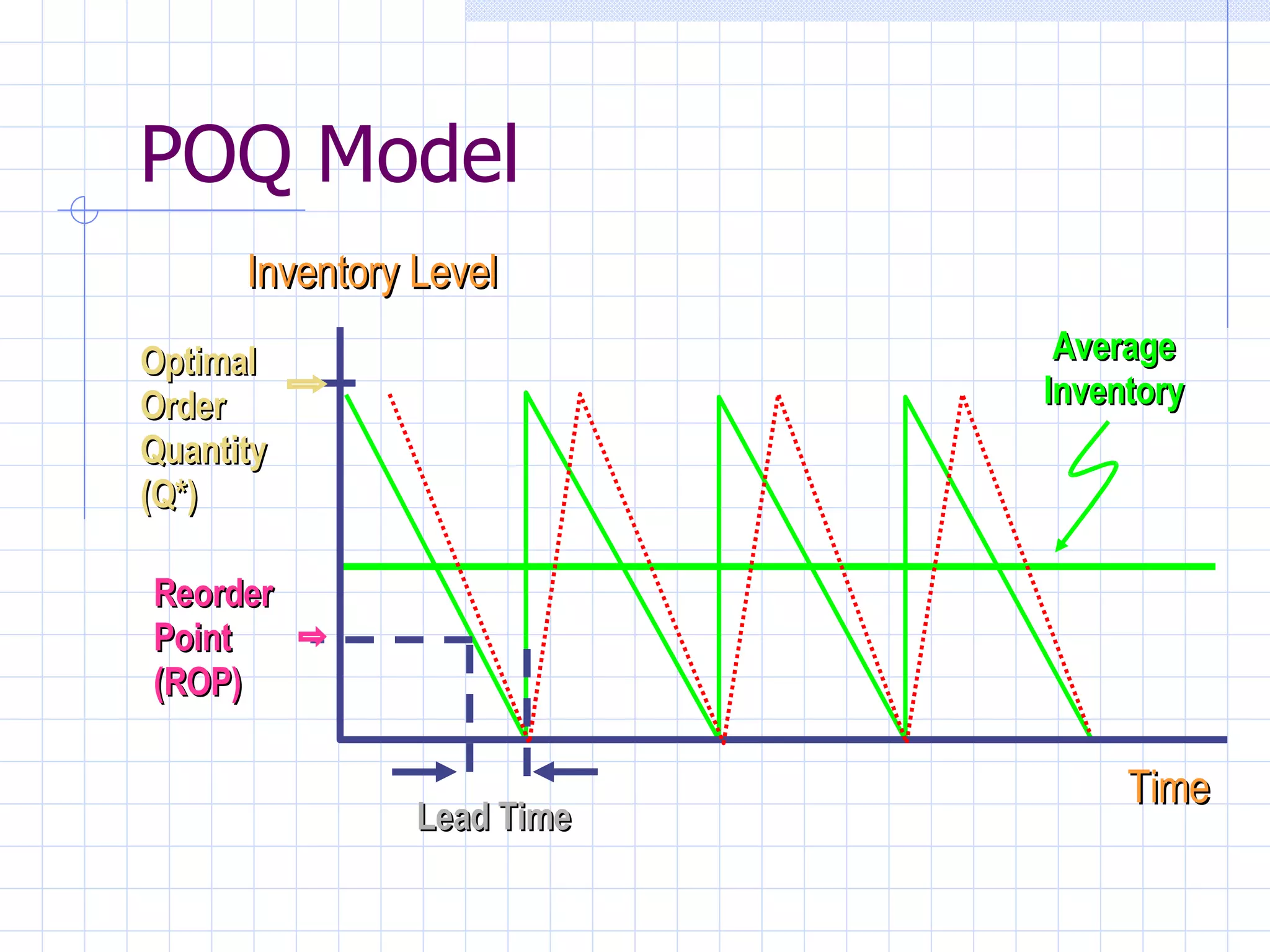
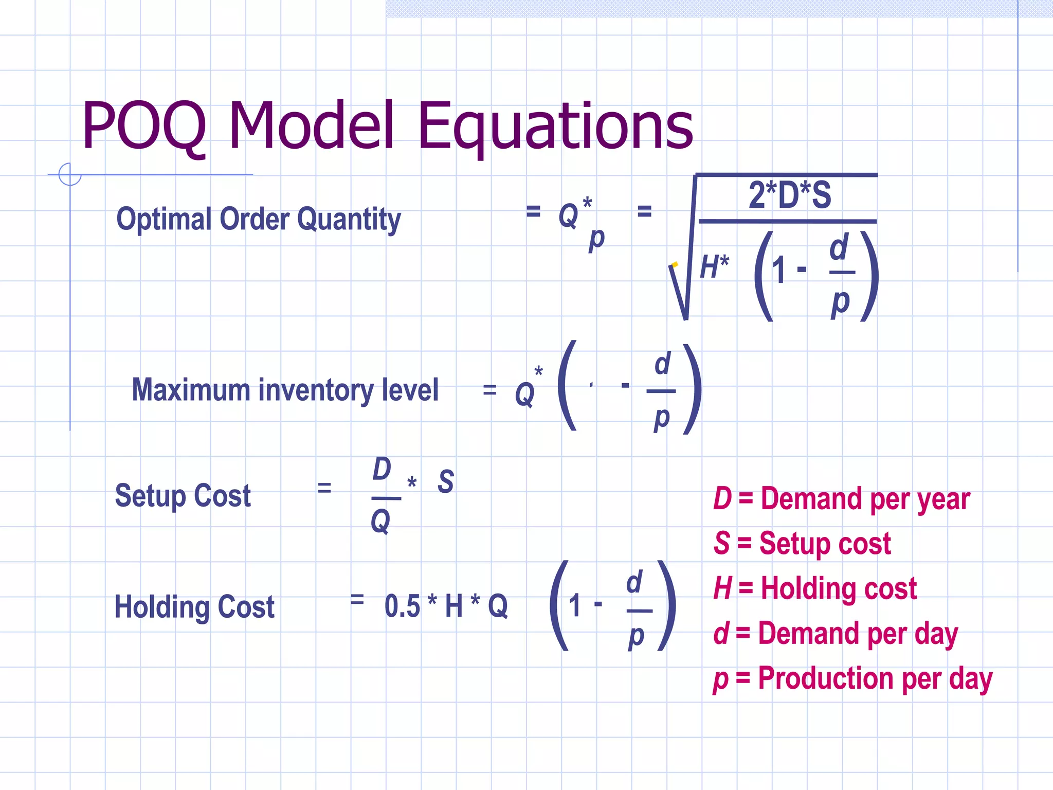
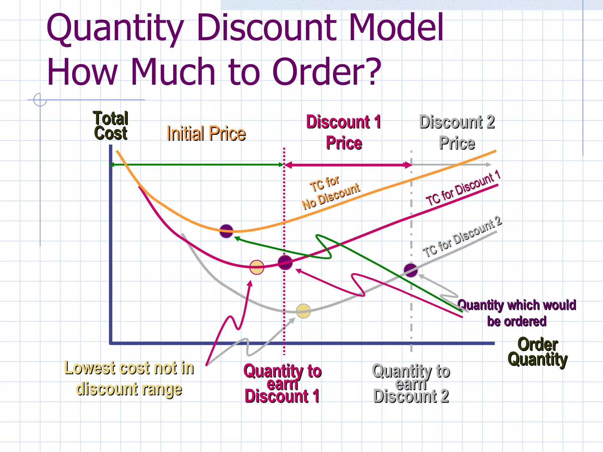
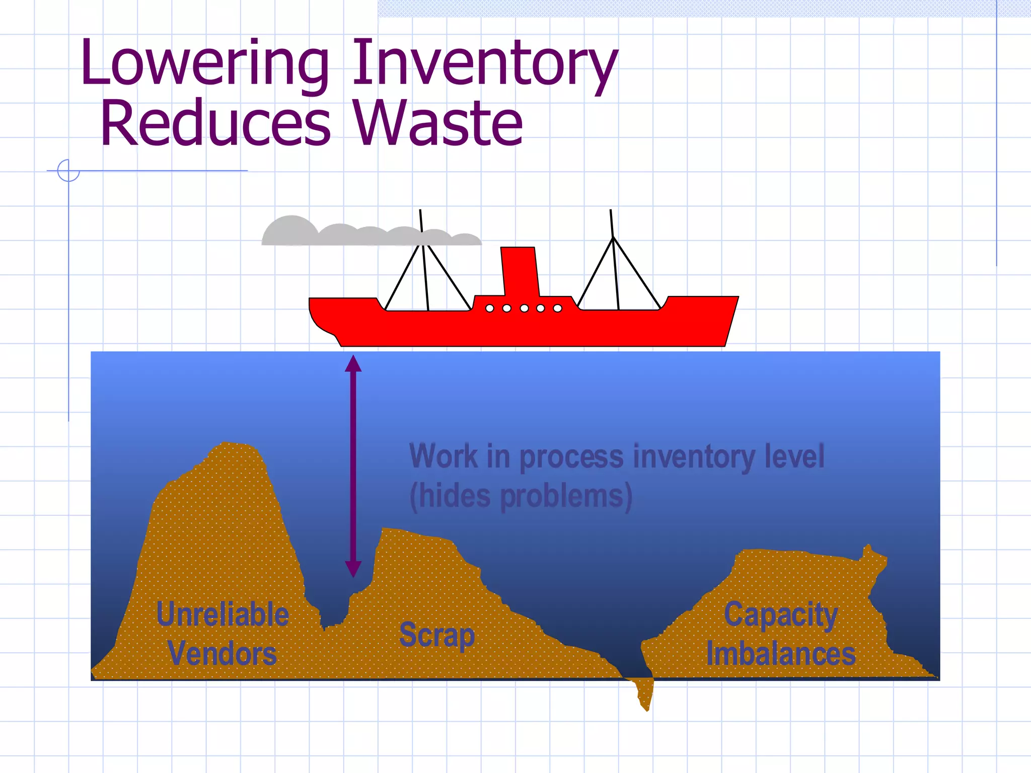
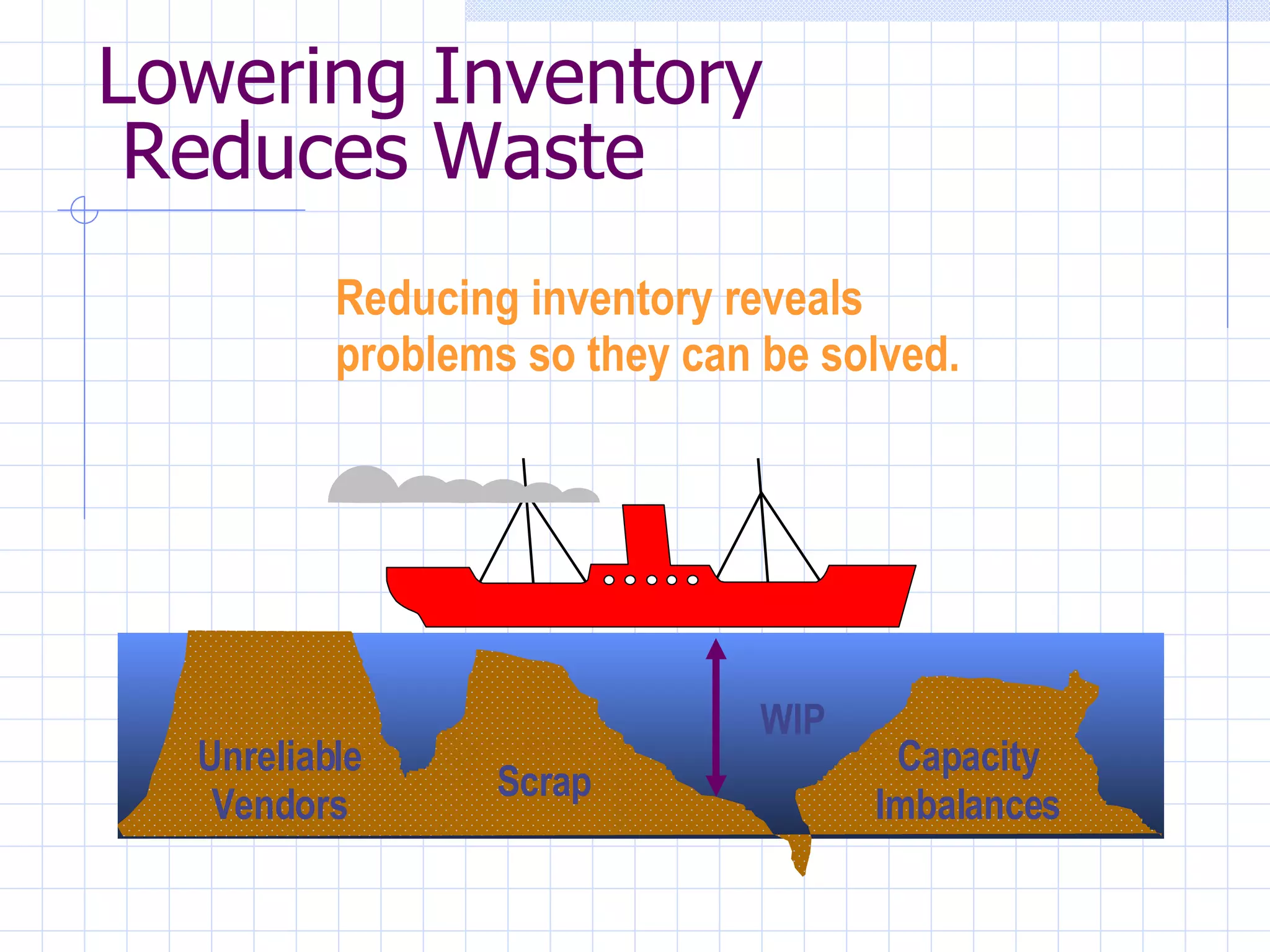
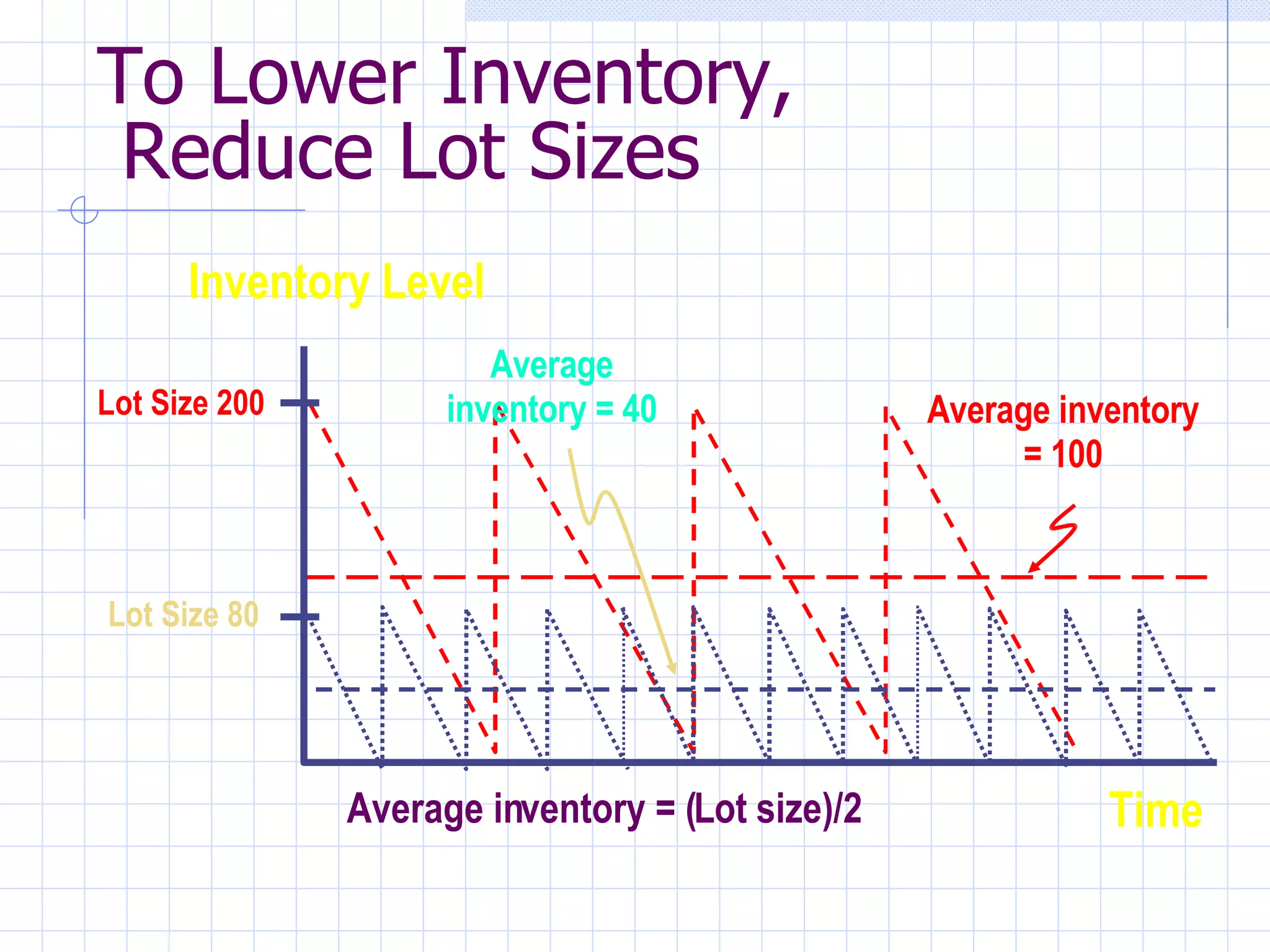
The document outlines various inventory management concepts including types of inventory, inventory classification systems, inventory models, and strategies for reducing inventory levels. It discusses direct and indirect inventory, ABC analysis, independent vs dependent demand, economic order quantity models, reorder points, probabilistic models, quantity discounts, fixed period systems, and how implementing just-in-time principles can help lower inventory through reducing lot sizes and setup times.

1. Outline for Managing Inventory Global Company Profile: Green Gear Cycling Functions of Inventory Types of Inventory Inventory Management ABC Analysis Record Accuracy Control of Service Inventory Inventory Models Independent versus Dependent Demand Holding, Ordering, and Setup Costs

2. Parts and materials Available capacity Human resources What is Inventory? © 1995 Corel Corp. © 1984-1994 T/Maker Co. © 1984-1994 T/Maker Co. © 1995 Corel Corp.

3. Green Gear Cycling Bike Friday - a bike in a suitcase Mass customization fast throughput low inventory work cells generalized machine (reduce setups) Balance between inventory holding cost and availability Aggressive attention to reducing cycle time of whole process

4. The Functions of Inventory To ”decouple” or separate various parts of the production process To provide a stock of goods that will provide a “selection” for customers To take advantage of quantity discounts To hedge against inflation and upward price changes

5. Inventory Classifications Inventory Process stage Demand Type Number & Value Other Raw Material WIP & Finished Goods Independent Dependent A Items B Items C Items Maintenance Dependent Operating

6. Types of Inventory Direct Inventory Raw material Work-in-progress (WIP) Finished goods Indirect Inventory Stored capacity Maintenance/repair/operating supply

7. Run time : Job is at machine and being worked on Setup time : Job is at the work station, and the work station is being "setup." Queue time : Job is where it should be, but is not being processed because other work precedes it. Move time : The time a job spends in transit Wait time : When one process is finished, but the job is waiting to be moved to the next work area. Other : "Just-in-case" inventory. The Material Flow Cycle and WIP Other Wait Time Move Time Queue Time Setup Time Run Time Input Cycle Time Output

8. Sources of Waste JIT “fights” seven types of waste Waste of motion --excessive or unnecessary human activity Waste of waiting --jobs waiting to be processed Waste of inventory --building up unnecessary inventory stocks Waste of conveyance --jobs being unnecessary moved Waste of processing --excessive or unnecessary operations Waste of overproduction --producing more than demanded Waste of correction ( defective products) --waste due to scrap, rework, repair, etc.

9. Independent vs. Dependent Demand Independent demand - demand for item is independent of demand for any other item EOQ Models Dependent demand - demand for item is dependent upon the demand for some other item MRP Systems

10. Higher costs Ordering (or setup) cost Costs of processing, clerks’ wages etc. Holding (or carrying) cost Building lease, insurance, opportunity, taxes etc. Difficult to control Hides production problems Disadvantages of Inventory

11. Inventory Tracking JIT and mass customization requires knowledge of location of all goods in order to precisely control the production plan Requires ERP data, barcode technology, RF and electronic communications to track inventory in transit, on the shop floor, and in the warehouse In JIT system, warehouse is less a warehouse than a “pass through facility.” Inaccurate inventory tracking is worse than no information

12. Holding Costs Breakdown (Approximate Ranges) Category Housing costs Material handling costs Labor and administration cost Investment costs Pilferage, scrap, and obsolescence Cost as a % of Inventory Value 6% (3 - 10% 3% (1 - 3.5%0 3% (3 - 5%) 11% (6 - 24%) 3% (2 - 5%)

13. EOQ Model: Minimize the overall Costs Order Quantity Cost Holding Cost Curve Total Cost Curve Ordering & Setup Costs Curve Optimal Order Quantity (Q*)

14. Inventory Holding Costs Obsolescence Insurance Extra staffing Interest Pilferage Damage Warehousing Etc.

15. Ordering Costs & Setup Costs Order processing Clerical support Clean-up costs Re-tooling costs Relocation or adjustment costs

16. Objective: Why holding cost increase? Why order cost decrease? Two underlying inventory question How much to order (e.g. finding EOQ) When to order (e.g. finding ROP)

17. Underline Decisions Supported by EOQ Models Objective: Minimizing the total inventory costs How much to order (Economic Order Quantity) When to order? (Reorder Point) How often should we place orders (Ordering Period) Others How to Take advantage of quantity discount What if the lead time and demand are not constant? Heuristics: Fixed Period Systems

18. Basic EOQ Model (Constant Demand and Lead Time) Reorder Point (ROP) Time Inventory Level Average Inventory (Q*/2) Lead Time Optimal Order Quantity (Q*)

19. Derive the EOQ: Finding Q* that Minimizes the Total Costs Total inventory cost = Order (Setup) cost + Holding cost To minimize TC, we set the derivative of TC with respect to Q* equal to 0 Thus,

20. EOQ Model Equations: How much to Order Optimal Order Quantity Expected Number of Orders Expected Time Between Orders Working Days / Year = = × × = = = = Q* D S H N D Q * T N 2 D = Demand per year S = Setup (order) cost per order H = Holding (carrying) cost

21. Reorder Point: When to Order? When there is lead time between order and delivery, we need to identify the reorder point to avoid out of stock. This provides answer for the second inventory “When to order?” ROP = (Demand per day)(Lead time for a new order in days) = d  L Working Days / Year = d D

22. EOQ Example Electronic Assembler, Inc. has to order 2920 TX5 circuit boards per year. The ordering cost is $80 per order; and the holding cost per unit per year is $50. The purchase price is $28. The items can be delivered in 5 days. The company would like to reduce its inventory costs by determining the optimal number of circuit boards to obtain per order. The conditions of ordering and inventory handling satisfy the assumptions of the EOQ model. Annual demand D = 2,920 units Daily demand d = 2,920/365=8 units Holding cost H = $50 per unit per year Ordering cost S = $80 per order Purchase price P = $28 per unit Lead time LT = 5 days Answer the following questions with detailed calculations and explanation: 1. Optimal quantity per order (EOQ): 2. Annual total relevant costs (optimal): 3. Annual total costs (optimal): 4. Number of orders per year: 5. Inventory cycle time (Nd=365 working days per year): 6. Reorder Point (ROP):

23. Allows partial receipt of material Other EOQ assumptions apply Suited for production environment Material produced, used immediately Provides production lot size Lower holding cost than EOQ model Production Order Quantity Model

24. POQ Model Reorder Point (ROP) Time Inventory Level Average Inventory Lead Time Optimal Order Quantity (Q*)

25. POQ Model Inventory Levels Inventory Leve l Time Supply Begins Supply Ends Production portion of cycle Demand portion of cycle with no supply

26. POQ Model Inventory Levels Time Inventory Level Production Portion of Cycle Max. Inventory Q·(1- d/p) Q* Supply Begins Supply Ends Inventory level with no demand Demand portion of cycle with no supply

27. POQ Model Equations D = Demand per year S = Setup cost H = Holding cost d = Demand per day p = Production per day Optimal Order Quantity Setup Cost Holding Cost = = - = * = * = Q H* d p Q D Q S p * 1 ( 0.5 * H * Q - d p 1 ) 1 ( ) 2*D*S ( ) Maximum inventory level - d p

28. Answers how much to order & when to order Allows quantity discounts Reduced price when item is purchased in larger quantities Other EOQ assumptions apply Trade-off is between lower price & increased holding cost Quantity Discount Model

29. Quantity Discount Model How Much to Order? Lowest cost not in discount range Order Quantity Total Cost Quantity which would be ordered TC for Discount 2 Quantity to earn Discount 2 Discount 2 Price Quantity to earn Discount 1 TC for Discount 1 Discount 1 Price TC for No Discount Initial Price

30. Allow demand and lead time to vary Follows normal distribution Other EOQ assumptions apply Consider service level & safety stock Service level = 1 - Probability of stockout Higher service level means more safety stock More safety stock means higher ROP Probabilistic Models

31. Probabilistic Models When to Order? Reorder Point (ROP) Optimal Order Quantity X Safety Stock (SS) Time Inventory Level Lead Time SS ROP Service Level P(Stockout) Place order Receive order Frequency

32. ABC Classification: Pareto Principle (Critical few and trivial many) 0 20 40 60 80 100 0 50 100 % of Inventory Items % Annual $ Usage A B C Class % $ Vol % Items A 80 15 B 15 30 C 5 55

33. Orders placed at fixed intervals Inventory brought up to target amount Amount ordered varies No continuous inventory count Possibility of stockout between intervals Useful when vendors visit routinely Example: P&G representative visits every 2 weeks Heuristics: Fixed Period Model

34. Heuristics: Fixed Period Model Time Inventory Level Target maximum Period Period Period

35. Traditional: inventory exists in case problems arise JIT objective: Eliminate redundant inventory JIT requires Small lot sizes Low setup time Containers for fixed number of parts JIT inventory: Minimum inventory to keep system running (lean but agile) Implementing JIT via Agile Inventory Management

36. Lowering Inventory Reduces Waste Scrap Work in process inventory level (hides problems) Unreliable Vendors Capacity Imbalances

37. Lowering Inventory Reduces Waste Scrap Reducing inventory reveals problems so they can be solved. Unreliable Vendors Capacity Imbalances WIP

38. To Lower Inventory, Reduce Lot Sizes Time Inventory Level Lot Size 200 Lot Size 80 Average inventory = 100 Average inventory = 40 Average inventory = (Lot size)/2

39. …Which Increases Inventory Costs Lot Size Cost Holding Cost Total Cost Setup Cost Optimal Lot Size Smaller Lot Size

40. Unless Setup Costs are Reduced Lot Size Cost Holding Cost Total Cost Original optimal lot size New optimal lot size Setup Cost

41. Steps to Reduce Setup Time (Honda Assembly Line) Initial Setup Time Separate setup into preparation, and actual setup, doing as much as possible while the machine/process is running (save 30 minutes) Move material closer and improve material handling (save 20 minutes) Standardize and improve tooling (save 15 minutes) 90 min 60 min 45 min 25 min 15 min Use one-touch system to eliminate adjustments (save 10 minutes) Training operators and standardizing work procedures (save 2 minutes) Step 1 Step 2 Step 3 Step 5 13 min Step 4

42. Reducing Lot Sizes Increases the Number of Lots Small lots increase flexibility to meet customer demands Strategies for eliminating waste and for eliminating waiting

43. Freeze Part of the Schedule A A B B B C JIT Small Lots Time A A B B B C Flexibility between Nissan plant and Dealers Five day before delivery: 100% flexibility Four day before: Freeze number of each model Three day before: Freeze change color Two day: Freeze major options One day before: Freeze minor options

44. Involves timing of operations JIT requires Communicating schedules to suppliers Level schedules Arrange flexible schedule for small lots (jelly bean scheduling) Freeze part of schedule nearest due date Kanban techniques JIT Scheduling

45. Japanese word for card Pronounced ‘kahn-bahn’ (not ‘can-ban’) Authorizes production from downstream operations ‘ Pulls’ material through plant May be a card, flag, verbal signal, empty container, real time message (stock broker, football player) etc. Most common example: use fixed-number containers or work permits to coordinate actions Add or remove containers to change production rate Kanban

46. Examples of Kanban