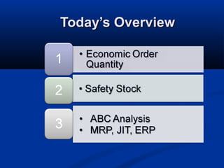
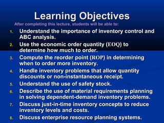
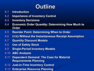
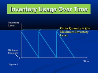
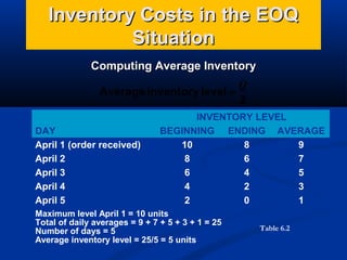
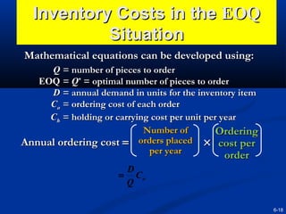
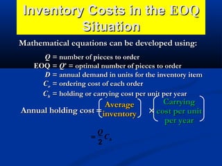
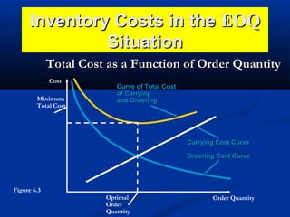
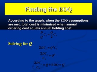
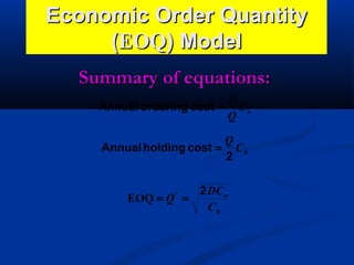
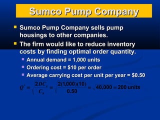
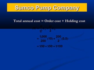
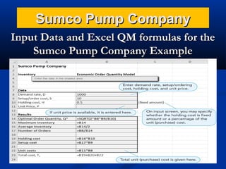
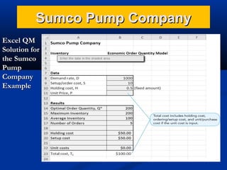
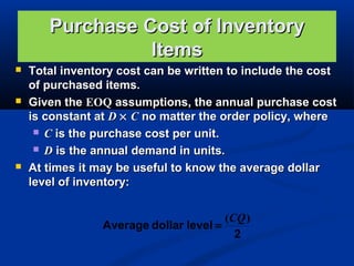
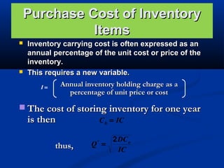
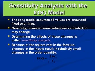
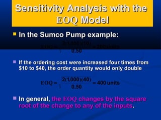
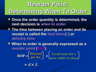
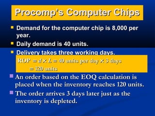
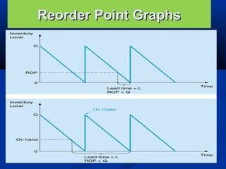
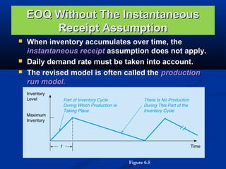
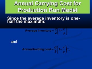
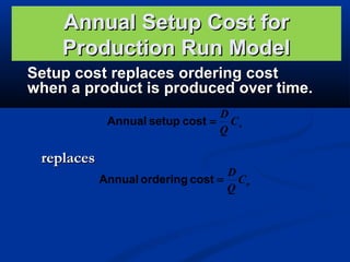
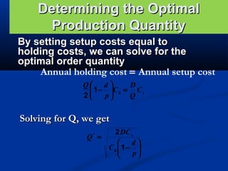
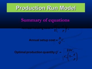
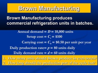
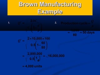
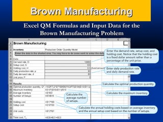
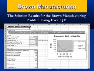
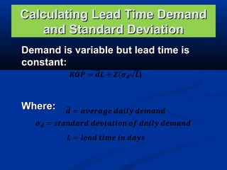
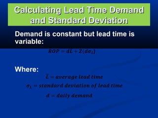
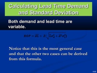
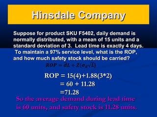
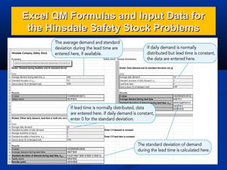
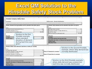
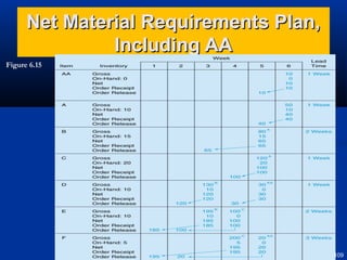
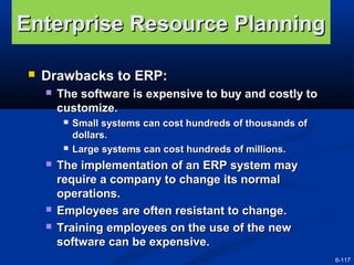
This document provides an overview of inventory control models and concepts. It discusses the economic order quantity (EOQ) model, which helps determine how much of an item to order to minimize total inventory costs. The EOQ balances ordering costs with carrying costs. The reorder point indicates when to place another order based on lead time and daily usage. Other topics covered include safety stock, material requirements planning, just-in-time inventory, and enterprise resource planning systems. Real-world examples are provided to demonstrate calculating the EOQ.

1. BBA3274 / DBS1084 QUANTITATIVE METHODS for BUSINESS
Inventory Control Models
Inventory Control Models
by
Stephen Ong
Visiting Fellow, Birmingham City
University Business School, UK
Visiting Professor, Shenzhen

2. Today’s Overview

3. Learning Objectives
After completing this lecture, students will be able to:
1.
2.
3.
4.
5.
6.
7.
8.
Understand the importance of inventory control and
ABC analysis.
Use the economic order quantity (EOQ) to
determine how much to order.
Compute the reorder point (ROP) in determining
when to order more inventory.
Handle inventory problems that allow quantity
discounts or non-instantaneous receipt.
Understand the use of safety stock.
Describe the use of material requirements planning
in solving dependent-demand inventory problems.
Discuss just-in-time inventory concepts to reduce
inventory levels and costs.
Discuss enterprise resource planning systems.

4. Outline
6.1
6.2
6.3
6.4
6.5
6.6
6.7
6.8
6.9
6.10
6.11
6.12
6.13
Introduction
Importance of Inventory Control
Inventory Decisions
Economic Order Quantity: Determining How Much to
Order
Reorder Point: Determining When to Order
EOQ Without the Instantaneous Receipt Assumption
Quantity Discount Models
Use of Safety Stock
Single-Period Inventory Models
ABC Analysis
Dependent Demand: The Case for Material
Requirements Planning
Just-in-Time Inventory Control
Enterprise Resource Planning

5. Introduction




Inventory is an expensive and important
asset to many companies.
Inventory is any stored resource used to
satisfy a current or future need.
Common examples are raw materials, workin-process, and finished goods.
Most companies try to balance high and low
inventory levels with cost minimization as a
goal.


Lower inventory levels can reduce costs.
Low inventory levels may result in stockouts and
dissatisfied customers.

6. Introduction




All organizations have some type of inventory
control system.
Inventory planning helps determine what
goods and/or services need to be produced.
Inventory planning helps determine whether
the organization produces the goods or
services or whether they are purchased from
another organization.
Inventory planning also involves demand
forecasting.

7. Introduction
Inventory planning and control
Planning on What
Inventory to Stock
and How to
Acquire It
Forecasting
Parts/Product
Demand
Controlling
Inventory
Levels
Feedback Measurements
to Revise Plans and
Forecasts
Figure 6.1
6-7

8. Importance of Inventory Control

Five uses of inventory:






The decoupling function
Storing resources
Irregular supply and demand
Quantity discounts
Avoiding stockouts and shortages
Decouple manufacturing processes.


Inventory is used as a buffer between stages
in a manufacturing process.
This reduces delays and improves efficiency.

9. Importance of Inventory Control

Storing resources.




Seasonal products may be stored to satisfy offseason demand.
Materials can be stored as raw materials, work-inprocess, or finished goods.
Labor can be stored as a component of partially
completed subassemblies.
Compensate for irregular supply and demand.


Demand and supply may not be constant over time.
Inventory can be used to buffer the variability.
6-9

10. Importance of Inventory Control

Take advantage of quantity discounts.
Lower prices may be available for larger
orders.
 Extra costs associated with holding more
inventory must be balanced against lower
purchase price.


Avoid stockouts and shortages.
Stockouts may result in lost sales.
 Dissatisfied customers may choose to buy
from another supplier.


11. Inventory Decisions

There are two fundamental decisions in
controlling inventory:




How much to order.
When to order.
The major objective is to minimize total
inventory costs.
Common inventory costs are:




Cost of the items (purchase or material cost).
Cost of ordering.
Cost of carrying, or holding, inventory.
Cost of stockouts.

12. Inventory Cost Factors
ORDERING COST FACTORS
CARRYING COST FACTORS
Developing and sending purchase
orders
Cost of capital
Processing and inspecting incoming
inventory
Taxes
Bill paying
Insurance
Inventory inquiries
Spoilage
Utilities, phone bills, and so on, for the
purchasing department
Theft
Salaries and wages for the purchasing
department employees
Obsolescence
Supplies, such as forms and paper, for Salaries and wages for warehouse
the purchasing department
employees
Utilities and building costs for the
warehouse
Table 6.1
Supplies, such as forms and paper, for
the warehouse

13. Inventory Cost Factors

Ordering costs are generally independent of
order quantity.



Carrying costs generally varies with the
amount of inventory, or the order size.


Many involve personnel time.
The amount of work is the same no matter the
size of the order.
The labour, space, and other costs increase as
the order size increases.
The actual cost of items purchased can vary
if there are quantity discounts available.

14. Economic Order Quantity
The economic order quantity
(EOQ) model is one of the oldest
and most commonly known
inventory control techniques.
 It is easy to use but has a
number of important
assumptions.
 Objective is to minimize total
cost of inventory.

6-14

15. Economic Order Quantity
Assumptions:
1.
2.
3.
4.
5.
6.
Demand is known and constant.
Lead time is known and constant.
Receipt of inventory is instantaneous.
Purchase cost per unit is constant throughout the
year.
The only variable costs are the cost of placing an
order, ordering cost, and the cost of holding or
storing inventory over time, holding or carrying
cost, and these are constant throughout the year.
Orders are placed so that stockouts or shortages
are avoided completely.

16. Inventory Usage Over Time
Inventory
Level
Order Quantity = Q =
Maximum Inventory
Level
Minimum
Inventory
0
Time
Figure 6.2

17. Inventory Costs in the EOQ
Situation
Computing Average Inventory
Q
Average inventory level =
2
DAY
April 1 (order received)
April 2
April 3
April 4
April 5
INVENTORY LEVEL
BEGINNING ENDING AVERAGE
10
8
9
8
6
7
6
4
5
4
2
3
2
0
1
Maximum level April 1 = 10 units
Total of daily averages = 9 + 7 + 5 + 3 + 1 = 25
Number of days = 5
Average inventory level = 25/5 = 5 units
Table 6.2

18. Inventory Costs in the EOQ
Situation
Mathematical equations can be developed using:
Q = number of pieces to order
EOQ = Q* = optimal number of pieces to order
D = annual demand in units for the inventory item
Co = ordering cost of each order
Ch = holding or carrying cost per unit per year
Number of
Ordering
Annual ordering cost = orders placed × cost per
per year
order
order
D
= Co
Q
6-18

19. Inventory Costs in the EOQ
Situation
Mathematical equations can be developed using:
Q = number of pieces to order
EOQ = Q* = optimal number of pieces to order
D = annual demand in units for the inventory item
Co = ordering cost of each order
Ch = holding or carrying cost per unit per year
Average
Annual holding cost = inventory
Q
= Ch
2
Carrying
× cost per unit
per year

20. Inventory Costs in the EOQ
Situation
Total Cost as a Function of Order Quantity
Cost
Minimum
Total Cost
Curve of Total Cost
of Carrying
and Ordering
Carrying Cost Curve
Ordering Cost Curve
Figure 6.3
Optimal
Order
Quantity
Order Quantity

21. Finding the EOQ
According to the graph, when the EOQ assumptions
are met, total cost is minimized when annual
ordering cost equals annual holding cost.
D
Q
Co = Ch
Q
2
Solving for Q
2 DC o = Q 2C h
2 DC o
= Q2
Ch
2 DC o
= Q = EOQ = Q *
Ch

22. Economic Order Quantity
(EOQ) Model
Summary of equations:
D
Annual ordering cost = C o
Q
Q
Annual holding cost = C h
2
EOQ = Q * =
2 DC o
Ch

23. Sumco Pump Company


Sumco Pump Company sells pump
housings to other companies.
The firm would like to reduce inventory
costs by finding optimal order quantity.



Annual demand = 1,000 units
Ordering cost = $10 per order
Average carrying cost per unit per year = $0.50
2 DC o
2(1,000 )(10)
Q =
=
= 40,000 = 200 units
Ch
0.50
*

24. Sumco Pump Company
Total annual cost = Order cost + Holding cost
D
Q
TC = C o + C h
Q
2
1,000
200
=
(10 ) +
(0.5 )
200
2
= $50 + $50 = $100

25. Sumco Pump Company
Input Data and Excel QM formulas for the
Sumco Pump Company Example

26. Sumco Pump Company
Excel QM
Solution for
the Sumco
Pump
Company
Example

27. Purchase Cost of Inventory
Items



Total inventory cost can be written to include the cost
of purchased items.
Given the EOQ assumptions, the annual purchase cost
is constant at D × C no matter the order policy, where
 C is the purchase cost per unit.
 D is the annual demand in units.
At times it may be useful to know the average dollar
level of inventory:
(CQ )
Average dollar level =
2

28. Purchase Cost of Inventory
Items


Inventory carrying cost is often expressed as an
annual percentage of the unit cost or price of the
inventory.
This requires a new variable.
Annual inventory holding charge as a
I=
percentage of unit price or cost
 The cost of storing inventory for one year
is then
thus,
C h = IC
2 DC o
Q =
IC
*

29. Sensitivity Analysis with the
EOQ Model




The EOQ model assumes all values are know and
fixed over time.
Generally, however, some values are estimated or
may change.
Determining the effects of these changes is
called sensitivity analysis.
Because of the square root in the formula,
changes in the inputs result in relatively small
changes in the order quantity.
2 DC o
EOQ =
Ch

30. Sensitivity Analysis with the
EOQ Model

In the Sumco Pump example:
2(1,000 )(10)
EOQ =
= 200 units
0.50
 If the ordering cost were increased four times from
$10 to $40, the order quantity would only double
2(1,000 )( 40)
EOQ =
= 400 units
0.50
 In general, the EOQ changes by the square
root of the change to any of the inputs.

31. Reorder Point:
Determining When To Order



Once the order quantity is determined, the
next decision is when to order.
The time between placing an order and its
receipt is called the lead time (L) or
delivery time.
When to order is generally expressed as a
reorder point (ROP).
Demand
Lead time for a
ROP = per day ×
new order in days
= d× L

32. Procomp’s Computer Chips



Demand for the computer chip is 8,000 per
year.
Daily demand is 40 units.
Delivery takes three working days.
ROP = d × L = 40 units per day × 3 days
= 120 units
 An order based on the EOQ calculation is
placed when the inventory reaches 120 units.
 The order arrives 3 days later just as the
inventory is depleted.

33. Reorder Point Graphs
Figure 6.4

34. EOQ Without The Instantaneous
Receipt Assumption



When inventory accumulates over time, the
instantaneous receipt assumption does not apply.
Daily demand rate must be taken into account.
The revised model is often called the production
run model.
Figure 6.5

35. Annual Carrying Cost for
Production Run Model


In production runs, setup cost replaces
ordering cost.
The model uses the following variables:
Q
= number of pieces per order, or
production run
Cs
= setup cost
Ch
= holding or carrying cost per unit per
year
p
= daily production rate
d
= daily demand rate
t= length of production run in days

36. Annual Carrying Cost for
Production Run Model
Maximum inventory level
= (Total produced during the production run)
– (Total used during the production run)
= (Daily production rate)(Number of days production)
– (Daily demand)(Number of days production)
= (pt) – (dt)
Total produced = Q = pt
since
we know
Q
t=
p
Maximum
Q
Q
 d
inventory = pt − dt = p − d = Q 1 − 
p
p
p

level

37. Annual Carrying Cost for
Production Run Model
Since the average inventory is onehalf the maximum:
Q d 
Average inventory =  1 − 
2
p
and
Q d 
Annual holding cost =  1 − C h
2
p

38. Annual Setup Cost for
Production Run Model
Setup cost replaces ordering cost
when a product is produced over time.
D
Annual setup cost = C s
Q
replaces
D
Annual ordering cost = C o
Q

39. Determining the Optimal
Production Quantity
By setting setup costs equal to
holding costs, we can solve for the
optimal order quantity
Annual holding cost = Annual setup cost
Q d 
D
 1 − C h = C s
2
p
Q
Solving for Q, we get
2 DC s
Q =
 d
C h  1− 
p

*

40. Production Run Model
Summary of equations
Q d 
Annual holding cost =  1 − C h
2
p
D
Annual setup cost = C s
Q
2 DC s
Optimal production quantity Q =
 d
C h  1− 
p

*

41. Brown Manufacturing
Brown Manufacturing produces
commercial refrigeration units in batches.
Annual demand = D = 10,000 units
Setup cost = Cs = $100
Carrying cost = Ch = $0.50 per unit per year
Daily production rate= p = 80 units daily
Daily demand rate = d = 60 units daily
1. How many units should Brown produce in each batch?
2. How long should the production part of the cycle last?

42. Brown Manufacturing
Example
1.
2 DC s
Q =
 d
C h  1− 
p

*
2 × 10,000 × 100
Q =
 60 
0.5 1 − 
 80 
2.
Q
Production cycle =
p
4,000
=
= 50 days
80
*
2,000,000
=
= 16,000,000
0.5 1
4
( )
= 4,000 units

43. Brown Manufacturing
Excel QM Formulas and Input Data for the
Brown Manufacturing Problem

44. Brown Manufacturing
The Solution Results for the Brown Manufacturing
Problem Using Excel QM

45. Quantity Discount Models


Quantity discounts are commonly available.
The basic EOQ model is adjusted by adding in the
purchase or materials cost.
Total cost = Material cost + Ordering cost + Holding cost
D
Q
Total cost = DC + C o + C h
Q
2
where
D=
Co =
C =
Ch =
annual demand in units
ordering cost of each order
cost per unit
holding or carrying cost per unit per year

46. Quantity Discount Models
Quantity unit cost is now variable,
Becausediscounts are commonly available.
 The basic EOQ model is adjusted by adding in the
Holding cost = Ch = IC
purchase or materials cost.

I = holding cost as a percentage of the unit cost (C)
Total cost = Material cost + Ordering cost + Holding cost
D
Q
Total cost = DC + C o + C h
Q
2
where
D = annual demand in units
Co = ordering cost of each order
C = cost per unit
Ch = holding or carrying cost per unit per year

47. Quantity Discount Models


A typical quantity discount schedule can
look like the table below.
However, buying at the lowest unit cost is
not always the best choice.
DISCOUNT
NUMBER
DISCOUNT
QUANTITY
DISCOUNT (%)
DISCOUNT
COST ($)
1
0 to 999
0
5.00
2
1,000 to 1,999
4
4.80
3
2,000 and over
5
4.75
Table 6.3

48. Quantity Discount Models
Total cost curve for the quantity discount model
Total
Cost
$
TC Curve for Discount 3
TC Curve for
Discount 1
TC Curve for Discount 2
EOQ for Discount 2
Figure 6.6
0
1,000
2,000
Order Quantity

49. Brass Department Store


Brass Department Store stocks toy race cars.
Their supplier has given them the quantity
discount schedule shown in Table 6.3.


Annual demand is 5,000 cars, ordering cost is $49, and
holding cost is 20% of the cost of the car
The first step is to compute EOQ values for each
discount.
(2)(5,000 )( 49)
EOQ 1 =
= 700 cars per order
(0.2)(5.00)
(2)(5,000 )( 49)
EOQ 2 =
= 714 cars per order
(0.2)( 4.80 )
(2)(5,000 )( 49)
EOQ 3 =
= 718 cars per order
(0.2)( 4.75 )

50. Brass Department Store
Example



The second step is adjust quantities below
the allowable discount range.
The EOQ for discount 1 is allowable.
The EOQs for discounts 2 and 3 are
outside the allowable range and have to be
adjusted to the smallest quantity possible
to purchase and receive the discount:
Q1 = 700
Q2 = 1,000
Q3 = 2,000

51. Brass Department Store
The third step is to compute the total cost for each
quantity.
ANNUAL
ORDERING
COST ($)
= (D/Q)Co
ANNUAL
CARRYING
COST ($)
= (Q/2)Ch
TOTAL ($)
DISCOUNT
NUMBER
UNIT
PRICE
(C )
ORDER
QUANTITY
(Q )
ANNUAL
MATERIAL
COST ($)
= DC
1
$5.00
700
25,000
350.00
350.00
25,700.00
2
4.80
1,000
24,000
245.00
480.00
24,725.00
3
4.75
2,000
23,750
122.50
950.00
24,822.50
The final step is to choose the
alternative with the lowest total cost.
Table 6.4

52. Brass Department Store
Excel QM’s Formulas and the Input Data for the Brass
Department Store Quantity Discount Problem

53. Brass Department Store
Excel QM’s Solution to the Brass
Department Store Problem

54. Use of Safety Stock




If demand or the lead time are uncertain,
the exact ROP will not be known with
certainty.
To prevent stockouts, it is necessary to
carry extra inventory called safety
stock.
Safety stock can prevent stockouts
when demand is unusually high.
Safety stock can be implemented by
adjusting the ROP.

55. Use of Safety Stock
 The
basic ROP equation is
ROP = d × L
d
=
daily demand (or average
daily demand)
L
=
order lead time or the
number of working days it takes to
deliver an order (or average lead time)
 A safety stock variable is added to the equation
to accommodate uncertain demand during lead
time
ROP = d × L + SS
where
SS = safety stock

56. Use of Safety Stock
Figure 6.7

57. ROP with Known Stockout
Costs




With a fixed EOQ and an ROP for placing
orders, stockouts can only occur during lead
time.
Our objective is to find the safety stock
quantity that will minimize the total of
stockout cost and holding cost.
We need to know the stockout cost per unit
and the probability distribution of demand
during lead time.
Estimating stockout costs can be difficult as
there may be direct and indirect costs.

58. Safety Stock with Unknown
Stockout Costs



There are many situations when stockout
costs are unknown.
An alternative approach to determining
safety stock levels is to use a service
level.
A service level is the percent of time you
will not be out of stock of a particular item.
Service level = 1 – Probability of a stockout
or
Probability of a stockout = 1 – Service level

59. Safety Stock with the Normal
Distribution
ROP = (Average Demand During Lead Time) + ZσdLT
Safety Stock = ZσdLT
Where:
Z = number of standard deviations for a
given service level
σdLT = standard deviation of demand
during lead time

60. Hinsdale Company



Inventory demand during lead time is normally
distributed.
Mean demand during lead time is 350 units with a
standard deviation of 10.
The company wants stockouts to occur only 5%
of the time.
µ = Mean demand = 350
σ dLT = Standard deviation = 10
X = Mean demand + Safety stock
SS = Safety stock = X – µ = Zσ
X −µ
Z=
σ
Figure 6.8
5% Area of
Normal Curve
SS
µ = 350
X= ?

61. Hinsdale Company Example

X − µ SS
=
From Appendix A we find Z = 1.65 =
σ
σ
 Solving for safety stock:
SS = 1.65(10) = 16.5 units, or 17 units
X = ROP = 350+16.5 = 366.5 units
5% Area of
Normal Curve
Figure 6.9
SS
µ = 350
X= ?

62. Hinsdale Company


Different safety stock levels will be generated for
different service levels.
However, the relationship is not linear.


You should be aware of what a service level is costing
in terms of carrying the safety stock in inventory.
The relationship between Z and safety stock can
be developed as follows:
X −µ
1. We know that Z =
σ
4. So we have
SS = Zσ
2. We also know that SS = X – µ
= Z(10)
SS
3. Thus Z = σ

63. Hinsdale Company
Safety Stock at different service levels
SERVICE
LEVEL (%)
90
91
92
93
94
95
96
97
98
Table 6.5
99
99.99
Z VALUE FROM
NORMAL CURVE TABLE
1.28
1.34
1.41
1.48
1.55
1.65
1.75
1.88
2.05
2.33
3.72
SAFETY STOCK
(UNITS)
12.8
13.4
14.1
14.8
15.5
16.5
17.5
18.8
20.5
23.3
37.2

64. Hinsdale Company
Service level versus annual carrying costs
This graph was
developed for a
specific case, but
the general shape
of the curve is the
same for all
service-level
problems.
Figure 6.9

65. Calculating Lead Time Demand
and Standard Deviation
 There
are three situations to
consider:
 Demand
is variable but lead time
is constant.
 Demand is constant but lead time
is variable.
 Both demand and lead time are
variable.

66. Calculating Lead Time Demand
and Standard Deviation
Demand is variable but lead time is
constant:
Where:

67. Calculating Lead Time Demand
and Standard Deviation
Demand is constant but lead time is
variable:
Where:

68. Calculating Lead Time Demand
and Standard Deviation
Both demand and lead time are
variable.
Notice that this is the most general case
and that the other two cases can be derived
from this formula.
6-68

69. Hinsdale Company
Suppose for product SKU F5402, daily demand is
normally distributed, with a mean of 15 units and a
standard deviation of 3. Lead time is exactly 4 days.
To maintain a 97% service level, what is the ROP,
and how much safety stock should be carried?
ROP = 15(4)+1.88(3*2)
= 60 + 11.28
=71.28
So the average demand during lead time
is 60 units, and safety stock is 11.28 units.

70. Hinsdale Company
Suppose for product SKU B7319, daily demand is
constant at 25 units per day, but lead time is
normally distributed, with a mean of 6 days and a
standard deviation of 3. To maintain a 98% service
level, what is the ROP?
ROP = 25(6)+2.05(25*3)
= 150+153.75
=303.75
So the average demand during lead time is 150
units, and safety stock is 153.75 units.

71. Hinsdale Company
Suppose for product SKU F9004, daily demand is
normally distributed, with a mean of 20 units and a
standard deviation of 4. Lead time is normally
distributed, with a mean of 5 days and a standard
deviation of 2 days. To maintain a 94% service
level, what is the ROP?
ROP = 100+1.55(40.99)
= 163.53

72. Calculating Annual Holding
Cost with Safety Stock
Under standard assumptions of
EOQ, average inventory is just Q/2.
 So annual holding cost is: (Q/2)*C .
h


This is not the case with safety
stock because safety stock is not
meant to be drawn down.

73. Calculating Annual Holding Cost
with Safety Stock
Total annual holding cost = holding
cost of regular inventory + holding
cost of safety stock
Where:
THC = total annual holding cost
Q = order quantity
Ch = holding cost per unit per year
SS = safety stock

74. Excel QM Formulas and Input Data for
the Hinsdale Safety Stock Problems

75. Excel QM Solution to the
Hinsdale Safety Stock Problem

76. Single-Period Inventory Models





Some products have no future value beyond the current
period.
These situations are called news vendor problems or
single-period inventory models.
Analysis uses marginal profit (MP) and marginal loss
(ML) and is called marginal analysis.
With a manageable number of states of nature and
alternatives, discrete distributions can be used.
When there are a large number of alternatives or states
of nature, the normal distribution may be used.

77. Marginal Analysis with
Discrete Distributions
We stock an additional unit only if the
expected marginal profit for that unit exceeds
the expected marginal loss.
P = probability that demand will be greater than
or equal to a given supply (or the
probability of selling at least one additional
unit).
1 – P = probability that demand will be less than
supply (or the probability that one
additional unit will not sell).

78. Marginal Analysis with
Discrete Distributions



The expected marginal profit is P(MP) .
The expected marginal loss is (1 – P)(ML).
The optimal decision rule is to stock the
additional unit if:
P(MP) ≥ (1 – P)ML
 With some basic manipulation:
P(MP) ≥ ML – P(ML)
P(MP) + P(ML) ≥ ML
P(MP + ML) ≥ ML
or
ML
P≥
ML + MP

79. Steps of Marginal Analysis
with Discrete Distributions
ML
1. Determine the value of
for the problem.
ML + MP
2. Construct a probability table and add a cumulative
probability column.
3. Keep ordering inventory as long as the probability
(P) of selling at least one additional
unit is greater than
ML
ML + MP

80. Café du Donut




The café buys donuts each day for $4 per carton
of 2 dozen donuts.
Any cartons not sold are thrown away at the end
of the day.
If a carton is sold, the total revenue is $6.
The marginal profit per carton is.
MP = Marginal profit = $6 – $4 = $2
 The marginal loss is $4 per carton since cartons
can not be returned or salvaged.

81. Café du Donut’s Probability
Distribution
DAILY SALES
(CARTONS OF DOUGHNUTS)
PROBABILITY (P) THAT DEMAND
WILL BE AT THIS LEVEL
4
5
0.05
0.15
6
7
0.15
0.20
8
9
0.25
0.10
10
0.10
1.00
Total
Table 6.6

82. Café du Donut Example
ML
Step 1. Determine the value of
for the
ML + MP
decision rule.
ML
$4
4
P≥
=
= = 0.67
ML + MP $4 + $2 6
P ≥ 0.67
Step 2.Add a new column to the table to
reflect the probability that doughnut
sales will be at each level or greater.

83. Marginal Analysis for Café
du Donut
DAILY SALES PROBABILITY (P)
(CARTONS OF THAT DEMAND WILL
DOUGHNUTS) BE AT THIS LEVEL
4
5
6
7
8
9
10
Total
Table 6.7
0.05
0.15
0.15
0.20
0.25
0.10
0.10
1.00
PROBABILITY (P) THAT
DEMAND WILL BE AT
THIS LEVEL OR
GREATER
1.00 ≥ 0.66
0.95 ≥ 0.66
0.80 ≥ 0.66
0.65
0.45
0.20
0.10

84. Café du Donut Example
Step 3. Keep ordering additional cartons as long
as the probability of selling at least one
additional carton is greater than P, which
is the indifference probability.
P at 6 cartons = 0.80 > 0.67

85. Marginal Analysis with the
Normal Distribution

We first need to find four values:
1.
2.
3.
4.
The average or mean sales for the product, µ
The standard deviation of sales, σ
The marginal profit for the product, MP.
The marginal loss for the product, ML.
 We let X * = optimal stocking level.

86. Steps of Marginal Analysis
with the Normal Distribution
1. Determine the value of
problem.
ML
for the
ML + MP
2. Locate P on the normal distribution (Appendix A)
and find the associated Z-value.
3. Find X * using the relationship:
Z=
X −µ
*
σ
to solve for the resulting stocking policy:
X = µ + Zσ
*

87. Joe’s Stocking Decision for
the Chicago Tribune


Demand for the Chicago Tribune at Joe’s Newsstand
averages 60 papers a day with a standard deviation of
10.
The marginal loss is 20 cents and the marginal profit
is 30 cents.
Step 1. Joe should stock the Tribune as long as
the probability of selling the last unit is at least
ML/(ML + MP):
ML
20 cents
20
=
=
= 0.40
ML + MP 20 cents + 30 cents 50
Let P = 0.40.

88. Joe’s Stocking Decision for
the Chicago Tribune
Step 2. Using the normal distribution in Figure
6.10, we find the appropriate Z value
Z = 0.25 standard deviations from the mean
Area under the Curve is 1 – 0.40 = 0.60
(Z = 0.25)
Mean Daily Sales
Area under the Curve is 0.40
Figure 6.10
µ = 50
X*
X = Demand
Optimal Stocking Policy (62 Newspapers)

89. Joe’s Stocking Decision for
the Chicago Tribune
Step 3. In this problem, µ = 60 and σ = 10,
so
X * − 60
0.25 =
10
or
X * = 60 + 0.25(10) = 62.5, or 62 newspapers
Joe should order 62 newspapers since
the probability of selling 63 newspapers
is slightly less than 0.40

90. Joe’s Stocking Decision for
the Chicago Tribune
 The procedure is the same when P > 0.50.
 Joe also stocks the Chicago Sun-Times.
 Marginal loss is 40 cents and marginal profit is 10 cents.
 Daily sales average 100 copies with a standard deviation
of 10 papers.
ML
40 cents
40
=
=
= 0.80
ML + MP 40 cents + 10 cents 50
 From Appendix A:
Z = – 0.84 standard deviations from the mean

91. Joe’s Stocking Decision for
the Chicago Tribune
With µ = 100 and σ = 10
X * − 100
− 0.84 =
10
or
X = 100 – 0.84(10)
= 91.6, or 91 newspapers
(Z = – 0.84)
*
Figure 6.11
Area under the
Curve is 0.40
X * µ = 100
Optimal Stocking Policy (91 Newspapers)
X = Demand

92. ABC Analysis


The purpose of ABC analysis is to divide the
inventory into three groups based on the overall
inventory value of the items.
Group A items account for the major portion of
inventory costs.



Group B items are more moderately priced.


Typically about 70% of the dollar value but only 10% of
the quantity of items.
Forecasting and inventory management must be done
carefully.
May represent 20% of the cost and 20% of the quantity.
Group C items are very low cost but high volume.

It is not cost effective to spend a lot of time managing
these items.

93. Summary of ABC Analysis
INVENTORY DOLLAR
GROUP
USAGE (%)
INVENTORY
ITEMS (%)
ARE QUANTITATIVE
CONTROL TECHNIQUES
USED?
A
70
10
Yes
B
20
20
In some cases
C
10
70
No
Table 6.8

94. Dependent Demand: The Case for
Material Requirements Planning



All the inventory models discussed so far
have assumed demand for one item is
independent of the demand for any other
item.
However, in many situations items demand is
dependent on demand for one or more other
items.
In these situations, Material Requirements
Planning (MRP) can be employed effectively.
6-94

95. Dependent Demand: The Case for
Material Requirements Planning

Some of the benefits of MRP are:
1.
2.
3.
4.
5.
6.

Increased customer service levels.
Reduced inventory costs.
Better inventory planning and scheduling.
Higher total sales.
Faster response to market changes and shifts.
Reduced inventory levels without reduced
customer service.
Most MRP systems are computerized, but
the basic analysis is straightforward.

96. Material Structure Tree




The first step is to develop a bill of materials
(BOM).
The BOM identifies components, descriptions,
and the number required for production of one
unit of the final product.
From the BOM we can develop a material
structure tree.
We use the following data:




Demand for product A is 50 units.
Each A requires 2 units of B and 3 units of C.
Each B requires 2 units of D and 3 units of E.
Each C requires 1 unit of E and 2 units of F.
6-96

97. Material Structure Tree
Material structure tree for Item A
Level
0
A
1
2
Figure 6.12
B(2)
D(2)
C(3)
E(3)
E(1)
F(2)

98. Material Structure Tree





It is clear from the three that the demand for B, C,
D, E, and F is completely dependent on the
demand for A.
The material structure tree has three levels: 0, 1,
and 2.
Items above a level are called parents.
Items below any level are called components.
The number in parenthesis beside each item
shows how many are required to make the item
above it.

99. Material Structure Tree
We can use the material structure tree and the
demand for Item A to compute demands for the other
items.
Part B:
Part C:
Part D:
Part E:
Part F:
2 × number of A’s = 2 × 50 = 100.
3 × number of A’s = 3 × 50 = 150.
2 × number of B’s = 2× 100 = 200.
3 × number of B’s + 1 × number of C’s = 3
× 100 + 1× 150 = 450.
2 × number of C’s = 2 × 150 = 300.

100. Gross and Net Material
Requirements Plan


Once the materials structure tree is done, we
construct a gross material requirements plan.
This is a time schedule that shows:



when an item must be ordered when there is no
inventory on hand, or
when the production of an item must be started in order
to satisfy the demand for the finished product at a
particular date.
We need lead times for each of the items.
Item A – 1 week
Item B – 2 weeks
Item C – 1 week
Item D – 1 week
Item E – 2 weeks
Item F – 3 weeks

101. Gross Material Requirements
Plan for 50 Units of A
Week
1
A
B
C
D
E
F
2
3
4
5
Required Date
50
Order Release
50
Required Date
100
Order Release
100
Required Date
150
Order Release
150
Required Date
200
Order Release
300
300
Required Date
Order Release
Lead Time = 1 Week
Lead Time = 2 Weeks
Lead Time = 1 Week
Lead Time = 1 Week
200
Required Date
Order Release
6
150
150
300
300
Figure 6.13
Lead Time = 2 Weeks
Lead Time = 3 Weeks

102. Net Material Requirements Plan
A net material requirements plan can be constructed
from the gross materials requirements plan and the
following on-hand inventory information:
ITEM
A
10
B
15
C
20
D
Table 6.9
ON-HAND INVENTORY
10
E
10
F
5

103. Net Material Requirements Plan

Using this data we can construct a plan
that includes:






Gross requirements.
On-hand inventory.
Net requirements.
Planned-order receipts.
Planned-order releases.
The net requirements plan is constructed
like the gross requirements plan.

104. Net Material Requirements
Plan for 50 Units of A
Week
A
1
2
3
4
5
Gross
On-Hand
10
6
50
Item
Lead
Time
1
10
Net
40
Order Receipt
40
Order Release
B
40
Gross
80A
On-Hand
15
15
Net
65
Order Receipt
65
Order Release
Figure 6.14(a)
65
2

105. Net Material Requirements
Plan for 50 Units of A
Week
Item
C
1
2
3
4
Gross
On-Hand
5
120A
20
1
10
Net
100
Order Receipt
100
Order Release
D
6
Lead
Time
100
Gross
On-Hand
130B
10
10
Net
120
Order Receipt
120
Order Release
Figure 6.14(b)
120
1

106. Net Material Requirements
Plan for 50 Units of A
Week
Item
3
4
195B
100C
10
0
Net
185
100
Order Receipt
E
1
185
100
Gross
On-Hand
10
Order Release
F
2
185
Gross
On-Hand
5
Net
195
Order Receipt
195
Order Release
Figure 6.14(c)
195
6
2
100
200C
5
5
Lead
Time
3

107. Two or More End Products


Most manufacturing companies have more than
one end item.
In this example, the second product is AA and it
has the following material structure tree:
AA
D(3)
F(2)
 If we require 10 units of AA, the gross requirements for
parts D and F can be computed:
Part D:
Part F:
3 × number of AA’s = 3 × 10 = 30
2 × number of AA’s = 2 × 10 = 20

108. Two or More End Products




The lead time for AA is one week.
The gross requirement for AA is 10 units in week 6
and there are no units on hand.
This new product can be added to the MRP
process.
The addition of AA will only change the MRP
schedules for the parts contained in AA.
 MRP can also schedule spare parts and
components.
 These have to be included as gross
requirements.

109. Net Material Requirements Plan,
Including AA
Figure 6.15
6-109

110. Just-in-Time (JIT) Inventory Control




To achieve greater efficiency in the
production process, organizations have
tried to have less in-process inventory on
hand.
This is known as JIT inventory.
The inventory arrives just in time to be
used during the manufacturing process.
One technique of implementing JIT is a
manual procedure called kanban.

111. Just-in-Time Inventory Control




Kanban in Japanese means “card.”
With a dual-card kanban system, there is a
conveyance kanban, or C-kanban, and a
production kanban, or P-kanban.
Kanban systems are quite simple, but they
require considerable discipline.
As there is little inventory to cover
variability, the schedule must be followed
exactly.

112. 4 Steps of Kanban
1.
2.
A user takes a container of parts or inventory
along with its C-kanban to his or her work area.
When there are no more parts or the container is
empty, the user returns the container along with
the C-kanban to the producer area.
At the producer area, there is a full container of
parts along with a P-kanban.
The user detaches the P-kanban from the full
container and takes the container and the Ckanban back to his or her area for immediate
use.

113. 4 Steps of Kanban
3.
4.
The detached P-kanban goes back to the
producer area along with the empty container
The P-kanban is a signal that new parts are to be
manufactured or that new parts are to be placed
in the container and is attached to the container
when it is filled .
This process repeats itself during the typical
workday.

114. The Kanban System
P-kanban
and
Container
C-kanban
and
Container
4
1
Producer
Area
Storage
Area
3
Figure 6.16
User
Area
2

115. Enterprise Resource Planning



MRP has evolved to include not only the materials
required in production, but also the labor hours,
material cost, and other resources related to
production.
In this approach the term MRP II is often used and
the word resource replaces the word requirements.
As this concept evolved and sophisticated software
was developed, these systems became known as
enterprise resource planning (ERP) systems.

116. Enterprise Resource Planning




The objective of an ERP System is to reduce costs
by integrating all of the operations of a firm.
Starts with the supplier of materials needed and
flows through the organization to include invoicing
the customer of the final product.
Data are entered only once into a database where it
can be quickly and easily accessed by anyone in the
organization.
Benefits include:
Reduced transaction costs.
 Increased speed and accuracy of
information.


117. Enterprise Resource Planning

Drawbacks to ERP:

The software is expensive to buy and costly to
customize.





Small systems can cost hundreds of thousands of
dollars.
Large systems can cost hundreds of millions.
The implementation of an ERP system may
require a company to change its normal
operations.
Employees are often resistant to change.
Training employees on the use of the new
software can be expensive.
6-117

118. Tutorial
Lab Practical : Spreadsheet
1 - 118

119. Further Reading



Render, B., Stair Jr.,R.M. & Hanna, M.E.
(2013) Quantitative Analysis for
Management, Pearson, 11th Edition
Waters, Donald (2007) Quantitative
Methods for Business, Prentice Hall, 4 th
Edition.
Anderson D, Sweeney D, & Williams T.
(2006) Quantitative Methods For
Business Thompson Higher Education,
10th Ed.

120. QUESTIONS?

References:

Inventory Control Models, 2013 Pearson Education, Inc. publishing as Prentice Hall
Special Inventory Models, 2010 Pearson Education, Inc. publishing as Prentice Hall
6.3 Further Business Applications: Economic Lot Size
Dr. Grethe Hystad, Mathematics Department, The University of Arizona (www.math.arizona.edu)
Business Dictionary (www.businessdictionary.com)
Inventory Control and Replacement Analysis Priyanshu
Hello Everyone!
This is the best ppt on 'Inventory Control and Replacement Analysis' that you can ever find.
I tried to include all the topics that will make the reader to grasp everything quickly.
These notes are also helpful for students for their university exams.
Go through the entire ppt and let me know your feedback in the comment box.
Learn and Enjoy!
Thank You!
INVENTORY MANAGEMENT
TECHNIQUES OF INVENTORY CONTROL
ECONOMIC ORDERING QUANTITY (EOQ)
Maximum Stock Level
Minimum Stock Level
Danger Level
ABC ANALYSIS FOR VALUE OF ITEMS
Perpetual Inventory System
H.M.L. Classification
F S N Analysis
V.E.D. Classification
Just in Time (JIT)
Inventory Turnover Ratio
WORKING CAPITAL MANAGEMENT
RECEIVABLES MANAGEMENT
COSTS OF MAINTAINING RECEIVABLES
BENEFITS OF MAINTAINING RECEIVABLES
FACTORS AFFECTING THE SIZE OF RECEIVABLES
CREDIT PERIOD
OPTIMUM SIZE OF RECEIVABLES
DETERMINANTS OF CREDIT POLICY
OPTIMUM CREDIT POLICY
Credit standards
Credit terms
CREDIT EVALUATION
Affordable Stationery Printing Services in Jaipur | Navpack n PrintNavpack & Print
Looking for professional printing services in Jaipur? Navpack n Print offers high-quality and affordable stationery printing for all your business needs. Stand out with custom stationery designs and fast turnaround times. Contact us today for a quote!
Attending a job Interview for B1 and B2 Englsih learnersErika906060
It is a sample of an interview for a business english class for pre-intermediate and intermediate english students with emphasis on the speking ability.
VAT Registration Outlined In UAE: Benefits and Requirementsuae taxgpt
Vat Registration is a legal obligation for businesses meeting the threshold requirement, helping companies avoid fines and ramifications. Contact now!
https://viralsocialtrends.com/vat-registration-outlined-in-uae/
Memorandum Of Association Constitution of Company.pptseri bangash
www.seribangash.com
A Memorandum of Association (MOA) is a legal document that outlines the fundamental principles and objectives upon which a company operates. It serves as the company's charter or constitution and defines the scope of its activities. Here's a detailed note on the MOA:
Contents of Memorandum of Association:
Name Clause: This clause states the name of the company, which should end with words like "Limited" or "Ltd." for a public limited company and "Private Limited" or "Pvt. Ltd." for a private limited company.
https://seribangash.com/article-of-association-is-legal-doc-of-company/
Registered Office Clause: It specifies the location where the company's registered office is situated. This office is where all official communications and notices are sent.
Objective Clause: This clause delineates the main objectives for which the company is formed. It's important to define these objectives clearly, as the company cannot undertake activities beyond those mentioned in this clause.
Liability Clause: It outlines the extent of liability of the company's members. In the case of companies limited by shares, the liability of members is limited to the amount unpaid on their shares. For companies limited by guarantee, members' liability is limited to the amount they undertake to contribute if the company is wound up.
https://seribangash.com/promotors-is-person-conceived-formation-company/
Capital Clause: This clause specifies the authorized capital of the company, i.e., the maximum amount of share capital the company is authorized to issue. It also mentions the division of this capital into shares and their respective nominal value.
Association Clause: It simply states that the subscribers wish to form a company and agree to become members of it, in accordance with the terms of the MOA.
Importance of Memorandum of Association:
Legal Requirement: The MOA is a legal requirement for the formation of a company. It must be filed with the Registrar of Companies during the incorporation process.
Constitutional Document: It serves as the company's constitutional document, defining its scope, powers, and limitations.
Protection of Members: It protects the interests of the company's members by clearly defining the objectives and limiting their liability.
External Communication: It provides clarity to external parties, such as investors, creditors, and regulatory authorities, regarding the company's objectives and powers.
https://seribangash.com/difference-public-and-private-company-law/
Binding Authority: The company and its members are bound by the provisions of the MOA. Any action taken beyond its scope may be considered ultra vires (beyond the powers) of the company and therefore void.
Amendment of MOA:
While the MOA lays down the company's fundamental principles, it is not entirely immutable. It can be amended, but only under specific circumstances and in compliance with legal procedures. Amendments typically require shareholder
LA HUG - Video Testimonials with Chynna Morgan - June 2024Lital Barkan
Have you ever heard that user-generated content or video testimonials can take your brand to the next level? We will explore how you can effectively use video testimonials to leverage and boost your sales, content strategy, and increase your CRM data.🤯
We will dig deeper into:
1. How to capture video testimonials that convert from your audience 🎥
2. How to leverage your testimonials to boost your sales 💲
3. How you can capture more CRM data to understand your audience better through video testimonials. 📊
Enterprise Excellence is Inclusive Excellence.pdfKaiNexus
Enterprise excellence and inclusive excellence are closely linked, and real-world challenges have shown that both are essential to the success of any organization. To achieve enterprise excellence, organizations must focus on improving their operations and processes while creating an inclusive environment that engages everyone. In this interactive session, the facilitator will highlight commonly established business practices and how they limit our ability to engage everyone every day. More importantly, though, participants will likely gain increased awareness of what we can do differently to maximize enterprise excellence through deliberate inclusion.
What is Enterprise Excellence?
Enterprise Excellence is a holistic approach that's aimed at achieving world-class performance across all aspects of the organization.
What might I learn?
A way to engage all in creating Inclusive Excellence. Lessons from the US military and their parallels to the story of Harry Potter. How belt systems and CI teams can destroy inclusive practices. How leadership language invites people to the party. There are three things leaders can do to engage everyone every day: maximizing psychological safety to create environments where folks learn, contribute, and challenge the status quo.
Who might benefit? Anyone and everyone leading folks from the shop floor to top floor.
Dr. William Harvey is a seasoned Operations Leader with extensive experience in chemical processing, manufacturing, and operations management. At Michelman, he currently oversees multiple sites, leading teams in strategic planning and coaching/practicing continuous improvement. William is set to start his eighth year of teaching at the University of Cincinnati where he teaches marketing, finance, and management. William holds various certifications in change management, quality, leadership, operational excellence, team building, and DiSC, among others.
"𝑩𝑬𝑮𝑼𝑵 𝑾𝑰𝑻𝑯 𝑻𝑱 𝑰𝑺 𝑯𝑨𝑳𝑭 𝑫𝑶𝑵𝑬"
𝐓𝐉 𝐂𝐨𝐦𝐬 (𝐓𝐉 𝐂𝐨𝐦𝐦𝐮𝐧𝐢𝐜𝐚𝐭𝐢𝐨𝐧𝐬) is a professional event agency that includes experts in the event-organizing market in Vietnam, Korea, and ASEAN countries. We provide unlimited types of events from Music concerts, Fan meetings, and Culture festivals to Corporate events, Internal company events, Golf tournaments, MICE events, and Exhibitions.
𝐓𝐉 𝐂𝐨𝐦𝐬 provides unlimited package services including such as Event organizing, Event planning, Event production, Manpower, PR marketing, Design 2D/3D, VIP protocols, Interpreter agency, etc.
Sports events - Golf competitions/billiards competitions/company sports events: dynamic and challenging
⭐ 𝐅𝐞𝐚𝐭𝐮𝐫𝐞𝐝 𝐩𝐫𝐨𝐣𝐞𝐜𝐭𝐬:
➢ 2024 BAEKHYUN [Lonsdaleite] IN HO CHI MINH
➢ SUPER JUNIOR-L.S.S. THE SHOW : Th3ee Guys in HO CHI MINH
➢FreenBecky 1st Fan Meeting in Vietnam
➢CHILDREN ART EXHIBITION 2024: BEYOND BARRIERS
➢ WOW K-Music Festival 2023
➢ Winner [CROSS] Tour in HCM
➢ Super Show 9 in HCM with Super Junior
➢ HCMC - Gyeongsangbuk-do Culture and Tourism Festival
➢ Korean Vietnam Partnership - Fair with LG
➢ Korean President visits Samsung Electronics R&D Center
➢ Vietnam Food Expo with Lotte Wellfood
"𝐄𝐯𝐞𝐫𝐲 𝐞𝐯𝐞𝐧𝐭 𝐢𝐬 𝐚 𝐬𝐭𝐨𝐫𝐲, 𝐚 𝐬𝐩𝐞𝐜𝐢𝐚𝐥 𝐣𝐨𝐮𝐫𝐧𝐞𝐲. 𝐖𝐞 𝐚𝐥𝐰𝐚𝐲𝐬 𝐛𝐞𝐥𝐢𝐞𝐯𝐞 𝐭𝐡𝐚𝐭 𝐬𝐡𝐨𝐫𝐭𝐥𝐲 𝐲𝐨𝐮 𝐰𝐢𝐥𝐥 𝐛𝐞 𝐚 𝐩𝐚𝐫𝐭 𝐨𝐟 𝐨𝐮𝐫 𝐬𝐭𝐨𝐫𝐢𝐞𝐬."
Unveiling the Secrets How Does Generative AI Work.pdfSam H
At its core, generative artificial intelligence relies on the concept of generative models, which serve as engines that churn out entirely new data resembling their training data. It is like a sculptor who has studied so many forms found in nature and then uses this knowledge to create sculptures from his imagination that have never been seen before anywhere else. If taken to cyberspace, gans work almost the same way.
RMD24 | Debunking the non-endemic revenue myth Marvin Vacquier Droop | First ...BBPMedia1
Marvin neemt je in deze presentatie mee in de voordelen van non-endemic advertising op retail media netwerken. Hij brengt ook de uitdagingen in beeld die de markt op dit moment heeft op het gebied van retail media voor niet-leveranciers.
Retail media wordt gezien als het nieuwe advertising-medium en ook mediabureaus richten massaal retail media-afdelingen op. Merken die niet in de betreffende winkel liggen staan ook nog niet in de rij om op de retail media netwerken te adverteren. Marvin belicht de uitdagingen die er zijn om echt aansluiting te vinden op die markt van non-endemic advertising.
Kseniya Leshchenko: Shared development support service model as the way to ma...Lviv Startup Club
Kseniya Leshchenko: Shared development support service model as the way to make small projects with small budgets profitable for the company (UA)
Kyiv PMDay 2024 Summer
Website – www.pmday.org
Youtube – https://www.youtube.com/startuplviv
FB – https://www.facebook.com/pmdayconference
Skye Residences | Extended Stay Residences Near Toronto Airportmarketingjdass
Experience unparalleled EXTENDED STAY and comfort at Skye Residences located just minutes from Toronto Airport. Discover sophisticated accommodations tailored for discerning travelers.
Website Link :
https://skyeresidences.com/
https://skyeresidences.com/about-us/
https://skyeresidences.com/gallery/
https://skyeresidences.com/rooms/
https://skyeresidences.com/near-by-attractions/
https://skyeresidences.com/commute/
https://skyeresidences.com/contact/
https://skyeresidences.com/queen-suite-with-sofa-bed/
https://skyeresidences.com/queen-suite-with-sofa-bed-and-balcony/
https://skyeresidences.com/queen-suite-with-sofa-bed-accessible/
https://skyeresidences.com/2-bedroom-deluxe-queen-suite-with-sofa-bed/
https://skyeresidences.com/2-bedroom-deluxe-king-queen-suite-with-sofa-bed/
https://skyeresidences.com/2-bedroom-deluxe-queen-suite-with-sofa-bed-accessible/
#Skye Residences Etobicoke, #Skye Residences Near Toronto Airport, #Skye Residences Toronto, #Skye Hotel Toronto, #Skye Hotel Near Toronto Airport, #Hotel Near Toronto Airport, #Near Toronto Airport Accommodation, #Suites Near Toronto Airport, #Etobicoke Suites Near Airport, #Hotel Near Toronto Pearson International Airport, #Toronto Airport Suite Rentals, #Pearson Airport Hotel Suites
Cracking the Workplace Discipline Code Main.pptxWorkforce Group
Cultivating and maintaining discipline within teams is a critical differentiator for successful organisations.
Forward-thinking leaders and business managers understand the impact that discipline has on organisational success. A disciplined workforce operates with clarity, focus, and a shared understanding of expectations, ultimately driving better results, optimising productivity, and facilitating seamless collaboration.
Although discipline is not a one-size-fits-all approach, it can help create a work environment that encourages personal growth and accountability rather than solely relying on punitive measures.
In this deck, you will learn the significance of workplace discipline for organisational success. You’ll also learn
• Four (4) workplace discipline methods you should consider
• The best and most practical approach to implementing workplace discipline.
• Three (3) key tips to maintain a disciplined workplace.