Downloaded 1,534 times


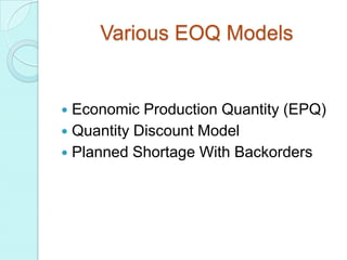
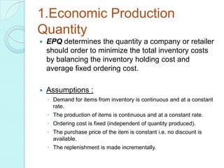
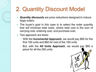
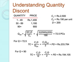
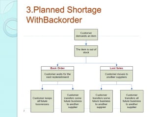
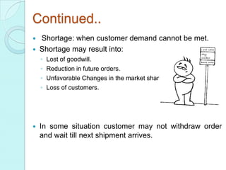
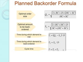


1. EOQ models determine the optimal order quantity to minimize total inventory costs by balancing ordering and holding costs. The basic EOQ formula considers constant demand, lead time, and costs. 2. Extensions of EOQ include EPQ, which accounts for continuous production, and quantity discount models, which optimize order size to receive lower per-unit prices. 3. Planned shortage models factor backorders, where unfulfilled customer demand is recorded and met by subsequent deliveries to minimize lost sales from stockouts. Formulas balance ordering, holding, and shortage costs.


