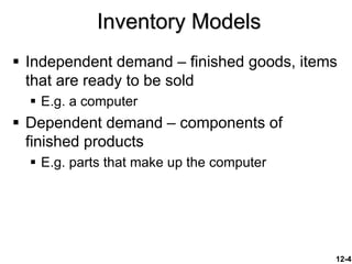
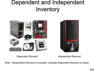
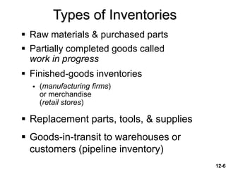
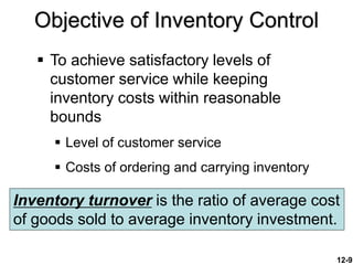
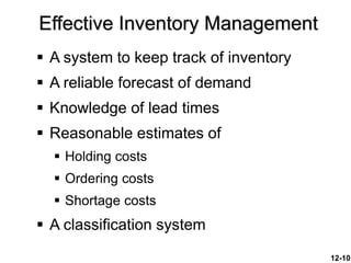
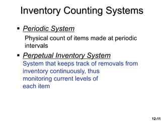
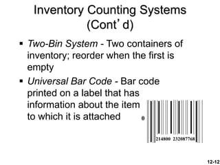
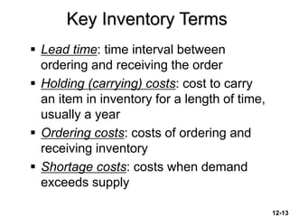
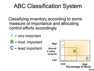
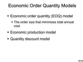
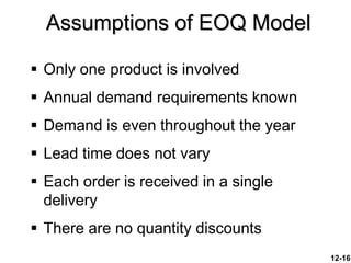
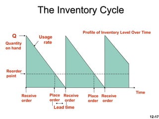
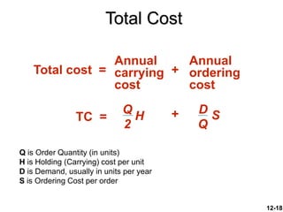
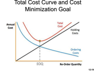
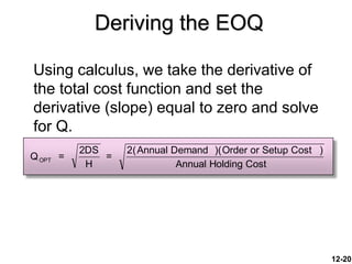
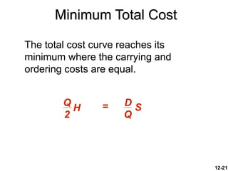
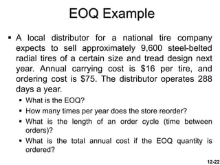
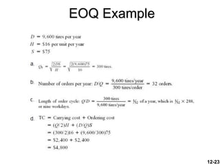
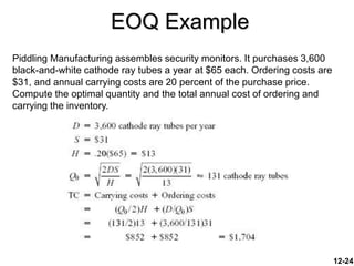
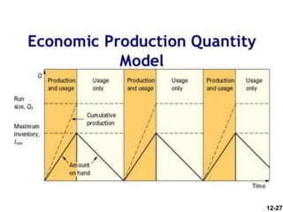
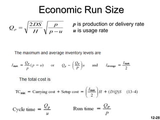
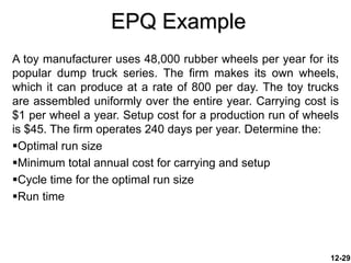
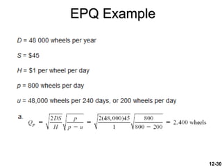
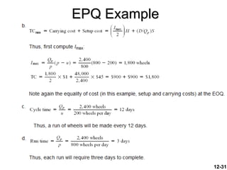
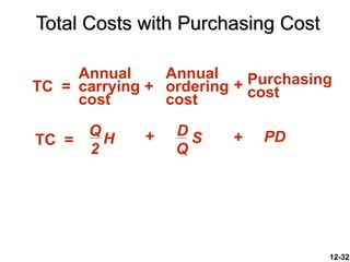
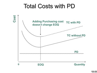
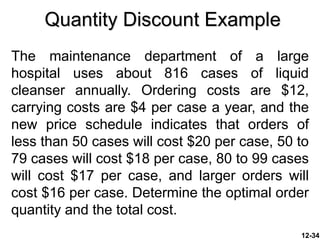
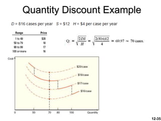
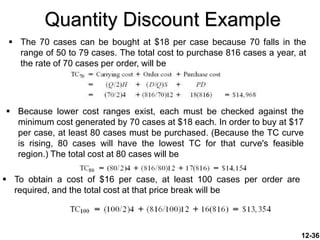
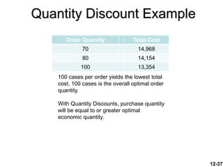
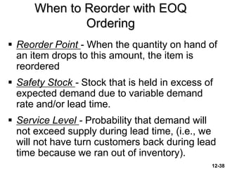
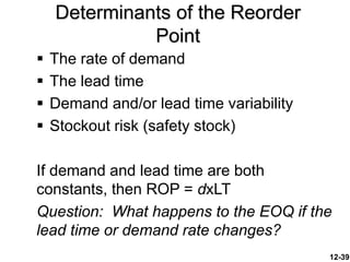
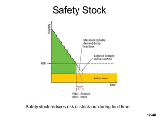
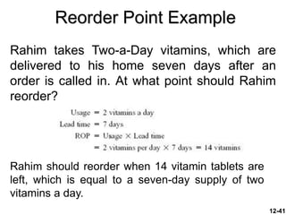
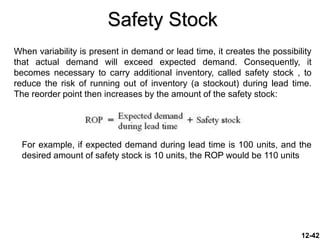
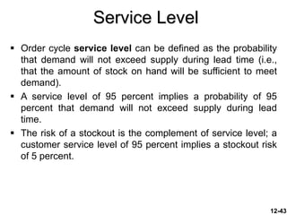
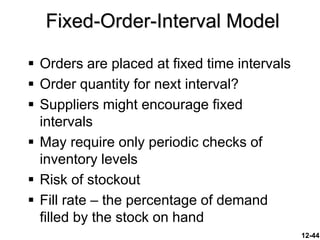
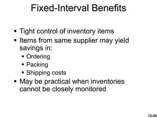
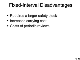
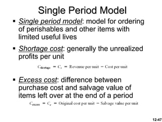
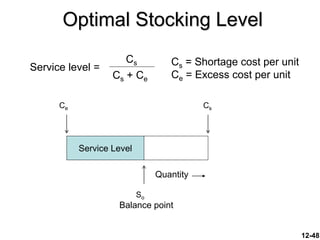
Stevenson
13
Inventory
Management
12-2
Learning Objectives
 Define the term inventory and list the major
reasons for holding inventories; and list the main
requirements for effective inventory management.
 Discuss the nature and importance of service
inventories
 Discuss periodic and perpetual review systems.
 Discuss the objectives of inventory management.
 Describe the A-B-C approach and explain how it
is useful.
12-3
Learning Objectives
 Describe the basic Economic Order Quantity
(“EOQ”) model and its assumptions, and solve
typical problems.
 Describe the Economic Production Quantity
(“EPQ”) model and solve typical problems.
 Describe the quantity discount model and solve
typical problems.
 Describe reorder point models and solve typical
problems.
12-4
Inventory Models
 Independent demand – finished goods, items
that are ready to be sold
 E.g. a computer
 Dependent demand – components of
finished products
 E.g. parts that make up the computer
12-5
Dependent and Independent
Inventory
Dependent Demand Independent Demand
Note: Independent Demand is uncertain, whereas Dependent Demand is certain
12-6
Types of Inventories
 Raw materials & purchased parts
 Partially completed goods called
work in progress
 Finished-goods inventories
 (manufacturing firms)
or merchandise
(retail stores)
 Replacement parts, tools, & supplies
 Goods-in-transit to warehouses or
customers (pipeline inventory)
12-7
Functions of Inventory
 To meet anticipated demand
 To smooth production requirements
 To decouple operations
 To protect against stock-outs
12-8
Functions of Inventory (Cont’d)
 To take advantage of order cycles
 To help hedge against price increases
 To permit operations
 To take advantage of quantity
discounts
12-9
Objective of Inventory Control
 To achieve satisfactory levels of
customer service while keeping
inventory costs within reasonable
bounds
 Level of customer service
 Costs of ordering and carrying inventory
Inventory turnover is the ratio of average cost
of goods sold to average inventory investment.
12-10
 A system to keep track of inventory
 A reliable forecast of demand
 Knowledge of lead times
 Reasonable estimates of
 Holding costs
 Ordering costs
 Shortage costs
 A classification system
Effective Inventory Management
12-11
Inventory Counting Systems
 Periodic System
Physical count of items made at periodic
intervals
 Perpetual Inventory System
System that keeps track of removals from
inventory continuously, thus
monitoring current levels of
each item
12-12
Inventory Counting Systems
(Cont’d)
 Two-Bin System - Two containers of
inventory; reorder when the first is
empty
 Universal Bar Code - Bar code
printed on a label that has
information about the item
to which it is attached 0
214800 232087768
12-13
 Lead time: time interval between
ordering and receiving the order
 Holding (carrying) costs: cost to carry
an item in inventory for a length of time,
usually a year
 Ordering costs: costs of ordering and
receiving inventory
 Shortage costs: costs when demand
exceeds supply
Key Inventory Terms
12-14
ABC Classification System
Classifying inventory according to some
measure of importance and allocating
control efforts accordingly.
A - very important
B - mod. important
C - least important Annual
$ value
of items
A
B
C
High
Low
Low High
Percentage of Items
12-15
 Economic order quantity (EOQ) model
 The order size that minimizes total annual
cost
 Economic production model
 Quantity discount model
Economic Order Quantity Models
12-16
 Only one product is involved
 Annual demand requirements known
 Demand is even throughout the year
 Lead time does not vary
 Each order is received in a single
delivery
 There are no quantity discounts
Assumptions of EOQ Model
12-17
The Inventory Cycle
Profile of Inventory Level Over Time
Quantity
on hand
Q
Receive
order
Place
order
Receive
order
Place
order
Receive
order
Lead time
Reorder
point
Usage
rate
Time
12-18
Total Cost
Annual
carrying
cost
Annual
ordering
cost
Total cost = +
TC =
Q
2
H
D
Q
S
+
Q is Order Quantity (in units)
H is Holding (Carrying) cost per unit
D is Demand, usually in units per year
S is Ordering Cost per order
Total Cost Curve and Cost
Minimization Goal
12-19
12-20
Deriving the EOQ
Using calculus, we take the derivative of
the total cost function and set the
derivative (slope) equal to zero and solve
for Q.
Q =
2DS
H
=
2(Annual Demand )(Order or Setup Cost )
Annual Holding Cost
OPT
12-21
Minimum Total Cost
The total cost curve reaches its
minimum where the carrying and
ordering costs are equal.
Q
2
H
D
Q
S
=
EOQ Example
12-22
 A local distributor for a national tire company
expects to sell approximately 9,600 steel-belted
radial tires of a certain size and tread design next
year. Annual carrying cost is $16 per tire, and
ordering cost is $75. The distributor operates 288
days a year.
 What is the EOQ?
 How many times per year does the store reorder?
 What is the length of an order cycle (time between
orders)?
 What is the total annual cost if the EOQ quantity is
ordered?
EOQ Example
12-23
EOQ Example
Piddling Manufacturing assembles security monitors. It purchases 3,600
black-and-white cathode ray tubes a year at $65 each. Ordering costs are
$31, and annual carrying costs are 20 percent of the purchase price.
Compute the optimal quantity and the total annual cost of ordering and
carrying the inventory.
12-24
12-25
 Production done in batches or lots
 Capacity to produce a part exceeds the
part’s usage or demand rate
 Assumptions of EPQ are similar to EOQ
except orders are received
incrementally during production
Economic Production Quantity (EPQ)
12-26
 Only one item is involved
 Annual demand is known
 Usage rate is constant
 Usage occurs continually
 Production rate is constant
 Lead time does not vary
 No quantity discounts
Economic Production Quantity
Assumptions
12-27
12-28
Economic Run Size
u
p
p
H
DS
Qp


2 p is production or delivery rate
u is usage rate
EPQ Example
A toy manufacturer uses 48,000 rubber wheels per year for its
popular dump truck series. The firm makes its own wheels,
which it can produce at a rate of 800 per day. The toy trucks
are assembled uniformly over the entire year. Carrying cost is
$1 per wheel a year. Setup cost for a production run of wheels
is $45. The firm operates 240 days per year. Determine the:
Optimal run size
Minimum total annual cost for carrying and setup
Cycle time for the optimal run size
Run time
12-29
EPQ Example
12-30
EPQ Example
12-31
12-32
Total Costs with Purchasing Cost
Annual
carrying
cost
Purchasing
cost
TC = +
Q
2
H
D
Q
S
TC = +
+
Annual
ordering
cost
PD
+
12-33
Total Costs with PD
Cost
EOQ
TC with PD
TC without PD
PD
0 Quantity
Adding Purchasing cost
doesn’t change EOQ
Quantity Discount Example
The maintenance department of a large
hospital uses about 816 cases of liquid
cleanser annually. Ordering costs are $12,
carrying costs are $4 per case a year, and the
new price schedule indicates that orders of
less than 50 cases will cost $20 per case, 50 to
79 cases will cost $18 per case, 80 to 99 cases
will cost $17 per case, and larger orders will
cost $16 per case. Determine the optimal order
quantity and the total cost.
12-34
Quantity Discount Example
12-35
Quantity Discount Example
 The 70 cases can be bought at $18 per case because 70 falls in the
range of 50 to 79 cases. The total cost to purchase 816 cases a year, at
the rate of 70 cases per order, will be
12-36
 Because lower cost ranges exist, each must be checked against the
minimum cost generated by 70 cases at $18 each. In order to buy at $17
per case, at least 80 cases must be purchased. (Because the TC curve
is rising, 80 cases will have the lowest TC for that curve's feasible
region.) The total cost at 80 cases will be
 To obtain a cost of $16 per case, at least 100 cases per order are
required, and the total cost at that price break will be
Quantity Discount Example
Order Quantity Total Cost
70 14,968
80 14,154
100 13,354
12-37
100 cases per order yields the lowest total
cost, 100 cases is the overall optimal order
quantity.
With Quantity Discounts, purchase quantity
will be equal to or greater optimal
economic quantity.
12-38
When to Reorder with EOQ
Ordering
 Reorder Point - When the quantity on hand of
an item drops to this amount, the item is
reordered
 Safety Stock - Stock that is held in excess of
expected demand due to variable demand
rate and/or lead time.
 Service Level - Probability that demand will
not exceed supply during lead time, (i.e., we
will not have turn customers back during lead
time because we ran out of inventory).
12-39
Determinants of the Reorder
Point
 The rate of demand
 The lead time
 Demand and/or lead time variability
 Stockout risk (safety stock)
If demand and lead time are both
constants, then ROP = dxLT
Question: What happens to the EOQ if the
lead time or demand rate changes?
12-40
Safety Stock
Safety stock reduces risk of stock-out during lead time
Reorder Point Example
Rahim takes Two-a-Day vitamins, which are
delivered to his home seven days after an
order is called in. At what point should Rahim
reorder?
12-41
Rahim should reorder when 14 vitamin tablets are
left, which is equal to a seven-day supply of two
vitamins a day.
Safety Stock
When variability is present in demand or lead time, it creates the possibility
that actual demand will exceed expected demand. Consequently, it
becomes necessary to carry additional inventory, called safety stock , to
reduce the risk of running out of inventory (a stockout) during lead time.
The reorder point then increases by the amount of the safety stock:
12-42
For example, if expected demand during lead time is 100 units, and the
desired amount of safety stock is 10 units, the ROP would be 110 units
Service Level
 Order cycle service level can be defined as the probability
that demand will not exceed supply during lead time (i.e.,
that the amount of stock on hand will be sufficient to meet
demand).
 A service level of 95 percent implies a probability of 95
percent that demand will not exceed supply during lead
time.
 The risk of a stockout is the complement of service level; a
customer service level of 95 percent implies a stockout risk
of 5 percent.
12-43
12-44
 Orders are placed at fixed time intervals
 Order quantity for next interval?
 Suppliers might encourage fixed
intervals
 May require only periodic checks of
inventory levels
 Risk of stockout
 Fill rate – the percentage of demand
filled by the stock on hand
Fixed-Order-Interval Model
12-45
 Tight control of inventory items
 Items from same supplier may yield
savings in:
 Ordering
 Packing
 Shipping costs
 May be practical when inventories
cannot be closely monitored
Fixed-Interval Benefits
12-46
 Requires a larger safety stock
 Increases carrying cost
 Costs of periodic reviews
Fixed-Interval Disadvantages
12-47
 Single period model: model for ordering
of perishables and other items with
limited useful lives
 Shortage cost: generally the unrealized
profits per unit
 Excess cost: difference between
purchase cost and salvage value of
items left over at the end of a period
Single Period Model
12-48
Optimal Stocking Level
Service Level
So
Quantity
Ce Cs
Balance point
Service level =
Cs
Cs + Ce
Cs = Shortage cost per unit
Ce = Excess cost per unit
12-49
Example
 Ce = $0.20 per unit
 Cs = $0.60 per unit
 Service level = Cs/(Cs+Ce) = .6/(.6+.2)
 Service level = .75
Service Level = 75%
Quantity
Ce Cs
Stockout risk = 1.00 – 0.75 = 0.25
12-50
 Too much inventory
 Tends to hide problems
 Easier to live with problems than to
eliminate them
 Costly to maintain
Operations Strategy

stevenson_chapter_13_-_inventory_management.ppt

  • 1.
  • 2.
    12-2 Learning Objectives  Definethe term inventory and list the major reasons for holding inventories; and list the main requirements for effective inventory management.  Discuss the nature and importance of service inventories  Discuss periodic and perpetual review systems.  Discuss the objectives of inventory management.  Describe the A-B-C approach and explain how it is useful.
  • 3.
    12-3 Learning Objectives  Describethe basic Economic Order Quantity (“EOQ”) model and its assumptions, and solve typical problems.  Describe the Economic Production Quantity (“EPQ”) model and solve typical problems.  Describe the quantity discount model and solve typical problems.  Describe reorder point models and solve typical problems.
  • 4.
    12-4 Inventory Models  Independentdemand – finished goods, items that are ready to be sold  E.g. a computer  Dependent demand – components of finished products  E.g. parts that make up the computer
  • 5.
    12-5 Dependent and Independent Inventory DependentDemand Independent Demand Note: Independent Demand is uncertain, whereas Dependent Demand is certain
  • 6.
    12-6 Types of Inventories Raw materials & purchased parts  Partially completed goods called work in progress  Finished-goods inventories  (manufacturing firms) or merchandise (retail stores)  Replacement parts, tools, & supplies  Goods-in-transit to warehouses or customers (pipeline inventory)
  • 7.
    12-7 Functions of Inventory To meet anticipated demand  To smooth production requirements  To decouple operations  To protect against stock-outs
  • 8.
    12-8 Functions of Inventory(Cont’d)  To take advantage of order cycles  To help hedge against price increases  To permit operations  To take advantage of quantity discounts
  • 9.
    12-9 Objective of InventoryControl  To achieve satisfactory levels of customer service while keeping inventory costs within reasonable bounds  Level of customer service  Costs of ordering and carrying inventory Inventory turnover is the ratio of average cost of goods sold to average inventory investment.
  • 10.
    12-10  A systemto keep track of inventory  A reliable forecast of demand  Knowledge of lead times  Reasonable estimates of  Holding costs  Ordering costs  Shortage costs  A classification system Effective Inventory Management
  • 11.
    12-11 Inventory Counting Systems Periodic System Physical count of items made at periodic intervals  Perpetual Inventory System System that keeps track of removals from inventory continuously, thus monitoring current levels of each item
  • 12.
    12-12 Inventory Counting Systems (Cont’d) Two-Bin System - Two containers of inventory; reorder when the first is empty  Universal Bar Code - Bar code printed on a label that has information about the item to which it is attached 0 214800 232087768
  • 13.
    12-13  Lead time:time interval between ordering and receiving the order  Holding (carrying) costs: cost to carry an item in inventory for a length of time, usually a year  Ordering costs: costs of ordering and receiving inventory  Shortage costs: costs when demand exceeds supply Key Inventory Terms
  • 14.
    12-14 ABC Classification System Classifyinginventory according to some measure of importance and allocating control efforts accordingly. A - very important B - mod. important C - least important Annual $ value of items A B C High Low Low High Percentage of Items
  • 15.
    12-15  Economic orderquantity (EOQ) model  The order size that minimizes total annual cost  Economic production model  Quantity discount model Economic Order Quantity Models
  • 16.
    12-16  Only oneproduct is involved  Annual demand requirements known  Demand is even throughout the year  Lead time does not vary  Each order is received in a single delivery  There are no quantity discounts Assumptions of EOQ Model
  • 17.
    12-17 The Inventory Cycle Profileof Inventory Level Over Time Quantity on hand Q Receive order Place order Receive order Place order Receive order Lead time Reorder point Usage rate Time
  • 18.
    12-18 Total Cost Annual carrying cost Annual ordering cost Total cost= + TC = Q 2 H D Q S + Q is Order Quantity (in units) H is Holding (Carrying) cost per unit D is Demand, usually in units per year S is Ordering Cost per order
  • 19.
    Total Cost Curveand Cost Minimization Goal 12-19
  • 20.
    12-20 Deriving the EOQ Usingcalculus, we take the derivative of the total cost function and set the derivative (slope) equal to zero and solve for Q. Q = 2DS H = 2(Annual Demand )(Order or Setup Cost ) Annual Holding Cost OPT
  • 21.
    12-21 Minimum Total Cost Thetotal cost curve reaches its minimum where the carrying and ordering costs are equal. Q 2 H D Q S =
  • 22.
    EOQ Example 12-22  Alocal distributor for a national tire company expects to sell approximately 9,600 steel-belted radial tires of a certain size and tread design next year. Annual carrying cost is $16 per tire, and ordering cost is $75. The distributor operates 288 days a year.  What is the EOQ?  How many times per year does the store reorder?  What is the length of an order cycle (time between orders)?  What is the total annual cost if the EOQ quantity is ordered?
  • 23.
  • 24.
    EOQ Example Piddling Manufacturingassembles security monitors. It purchases 3,600 black-and-white cathode ray tubes a year at $65 each. Ordering costs are $31, and annual carrying costs are 20 percent of the purchase price. Compute the optimal quantity and the total annual cost of ordering and carrying the inventory. 12-24
  • 25.
    12-25  Production donein batches or lots  Capacity to produce a part exceeds the part’s usage or demand rate  Assumptions of EPQ are similar to EOQ except orders are received incrementally during production Economic Production Quantity (EPQ)
  • 26.
    12-26  Only oneitem is involved  Annual demand is known  Usage rate is constant  Usage occurs continually  Production rate is constant  Lead time does not vary  No quantity discounts Economic Production Quantity Assumptions
  • 27.
  • 28.
    12-28 Economic Run Size u p p H DS Qp   2p is production or delivery rate u is usage rate
  • 29.
    EPQ Example A toymanufacturer uses 48,000 rubber wheels per year for its popular dump truck series. The firm makes its own wheels, which it can produce at a rate of 800 per day. The toy trucks are assembled uniformly over the entire year. Carrying cost is $1 per wheel a year. Setup cost for a production run of wheels is $45. The firm operates 240 days per year. Determine the: Optimal run size Minimum total annual cost for carrying and setup Cycle time for the optimal run size Run time 12-29
  • 30.
  • 31.
  • 32.
    12-32 Total Costs withPurchasing Cost Annual carrying cost Purchasing cost TC = + Q 2 H D Q S TC = + + Annual ordering cost PD +
  • 33.
    12-33 Total Costs withPD Cost EOQ TC with PD TC without PD PD 0 Quantity Adding Purchasing cost doesn’t change EOQ
  • 34.
    Quantity Discount Example Themaintenance department of a large hospital uses about 816 cases of liquid cleanser annually. Ordering costs are $12, carrying costs are $4 per case a year, and the new price schedule indicates that orders of less than 50 cases will cost $20 per case, 50 to 79 cases will cost $18 per case, 80 to 99 cases will cost $17 per case, and larger orders will cost $16 per case. Determine the optimal order quantity and the total cost. 12-34
  • 35.
  • 36.
    Quantity Discount Example The 70 cases can be bought at $18 per case because 70 falls in the range of 50 to 79 cases. The total cost to purchase 816 cases a year, at the rate of 70 cases per order, will be 12-36  Because lower cost ranges exist, each must be checked against the minimum cost generated by 70 cases at $18 each. In order to buy at $17 per case, at least 80 cases must be purchased. (Because the TC curve is rising, 80 cases will have the lowest TC for that curve's feasible region.) The total cost at 80 cases will be  To obtain a cost of $16 per case, at least 100 cases per order are required, and the total cost at that price break will be
  • 37.
    Quantity Discount Example OrderQuantity Total Cost 70 14,968 80 14,154 100 13,354 12-37 100 cases per order yields the lowest total cost, 100 cases is the overall optimal order quantity. With Quantity Discounts, purchase quantity will be equal to or greater optimal economic quantity.
  • 38.
    12-38 When to Reorderwith EOQ Ordering  Reorder Point - When the quantity on hand of an item drops to this amount, the item is reordered  Safety Stock - Stock that is held in excess of expected demand due to variable demand rate and/or lead time.  Service Level - Probability that demand will not exceed supply during lead time, (i.e., we will not have turn customers back during lead time because we ran out of inventory).
  • 39.
    12-39 Determinants of theReorder Point  The rate of demand  The lead time  Demand and/or lead time variability  Stockout risk (safety stock) If demand and lead time are both constants, then ROP = dxLT Question: What happens to the EOQ if the lead time or demand rate changes?
  • 40.
    12-40 Safety Stock Safety stockreduces risk of stock-out during lead time
  • 41.
    Reorder Point Example Rahimtakes Two-a-Day vitamins, which are delivered to his home seven days after an order is called in. At what point should Rahim reorder? 12-41 Rahim should reorder when 14 vitamin tablets are left, which is equal to a seven-day supply of two vitamins a day.
  • 42.
    Safety Stock When variabilityis present in demand or lead time, it creates the possibility that actual demand will exceed expected demand. Consequently, it becomes necessary to carry additional inventory, called safety stock , to reduce the risk of running out of inventory (a stockout) during lead time. The reorder point then increases by the amount of the safety stock: 12-42 For example, if expected demand during lead time is 100 units, and the desired amount of safety stock is 10 units, the ROP would be 110 units
  • 43.
    Service Level  Ordercycle service level can be defined as the probability that demand will not exceed supply during lead time (i.e., that the amount of stock on hand will be sufficient to meet demand).  A service level of 95 percent implies a probability of 95 percent that demand will not exceed supply during lead time.  The risk of a stockout is the complement of service level; a customer service level of 95 percent implies a stockout risk of 5 percent. 12-43
  • 44.
    12-44  Orders areplaced at fixed time intervals  Order quantity for next interval?  Suppliers might encourage fixed intervals  May require only periodic checks of inventory levels  Risk of stockout  Fill rate – the percentage of demand filled by the stock on hand Fixed-Order-Interval Model
  • 45.
    12-45  Tight controlof inventory items  Items from same supplier may yield savings in:  Ordering  Packing  Shipping costs  May be practical when inventories cannot be closely monitored Fixed-Interval Benefits
  • 46.
    12-46  Requires alarger safety stock  Increases carrying cost  Costs of periodic reviews Fixed-Interval Disadvantages
  • 47.
    12-47  Single periodmodel: model for ordering of perishables and other items with limited useful lives  Shortage cost: generally the unrealized profits per unit  Excess cost: difference between purchase cost and salvage value of items left over at the end of a period Single Period Model
  • 48.
    12-48 Optimal Stocking Level ServiceLevel So Quantity Ce Cs Balance point Service level = Cs Cs + Ce Cs = Shortage cost per unit Ce = Excess cost per unit
  • 49.
    12-49 Example  Ce =$0.20 per unit  Cs = $0.60 per unit  Service level = Cs/(Cs+Ce) = .6/(.6+.2)  Service level = .75 Service Level = 75% Quantity Ce Cs Stockout risk = 1.00 – 0.75 = 0.25
  • 50.
    12-50  Too muchinventory  Tends to hide problems  Easier to live with problems than to eliminate them  Costly to maintain Operations Strategy