Download as PDF, PPTX

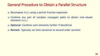
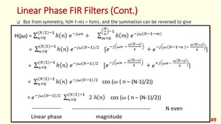
![Linear Time-Invariant Digital Filters (Cont.)
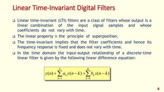
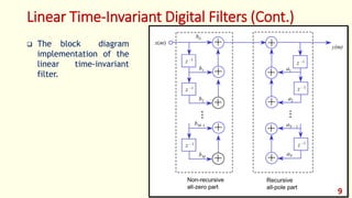
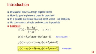
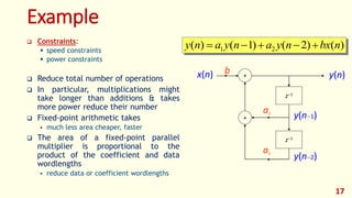
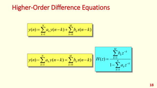
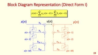
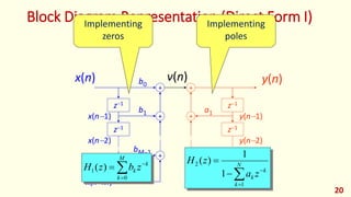
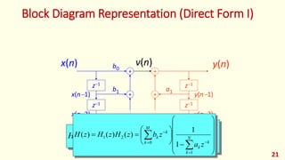
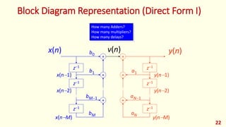
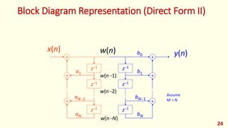
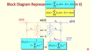
Where {𝑎 𝑘 , 𝑏 𝑘} are the filter coefficients, and the output 𝑦(𝑛) is a linear
combination of the previous 𝑁 output samples [𝑦(𝑛 − 1), … , 𝑦(𝑛 − 𝑁)], the present
input sample 𝑥(𝑛) and the previous 𝑀 input samples [𝑥(𝑛 − 1), … , 𝑥(𝑛 − 𝑀)].
The characteristic of a filter is completely determined by its coefficients
{𝑎 𝑘 , 𝑏 𝑘}.
For a time-invariant filter the coefficients {𝑎 𝑘 , 𝑏 𝑘} are constants calculated
to obtain a specified frequency response.
M
k
k
N
k
k knxbknyany
01
)()()(
5](https://image.slidesharecdn.com/dspfoehu-lec07-digitalfilters-170328231257/85/DSP_FOEHU-Lec-07-Digital-Filters-5-320.jpg)
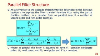
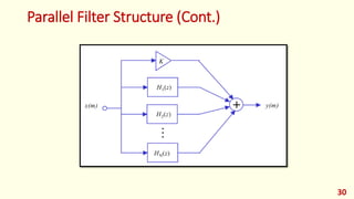


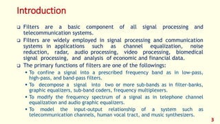
The document discusses digital filters and their design. It begins with an introduction to filters and their uses in signal processing applications. It then covers linear time-invariant filters and their transfer functions. It discusses the differences between non-recursive (FIR) and recursive (IIR) filters. The document presents various filter structures for implementation, including direct form I and direct form II structures. It also discusses designing FIR and IIR filters as well as issues in their implementation.