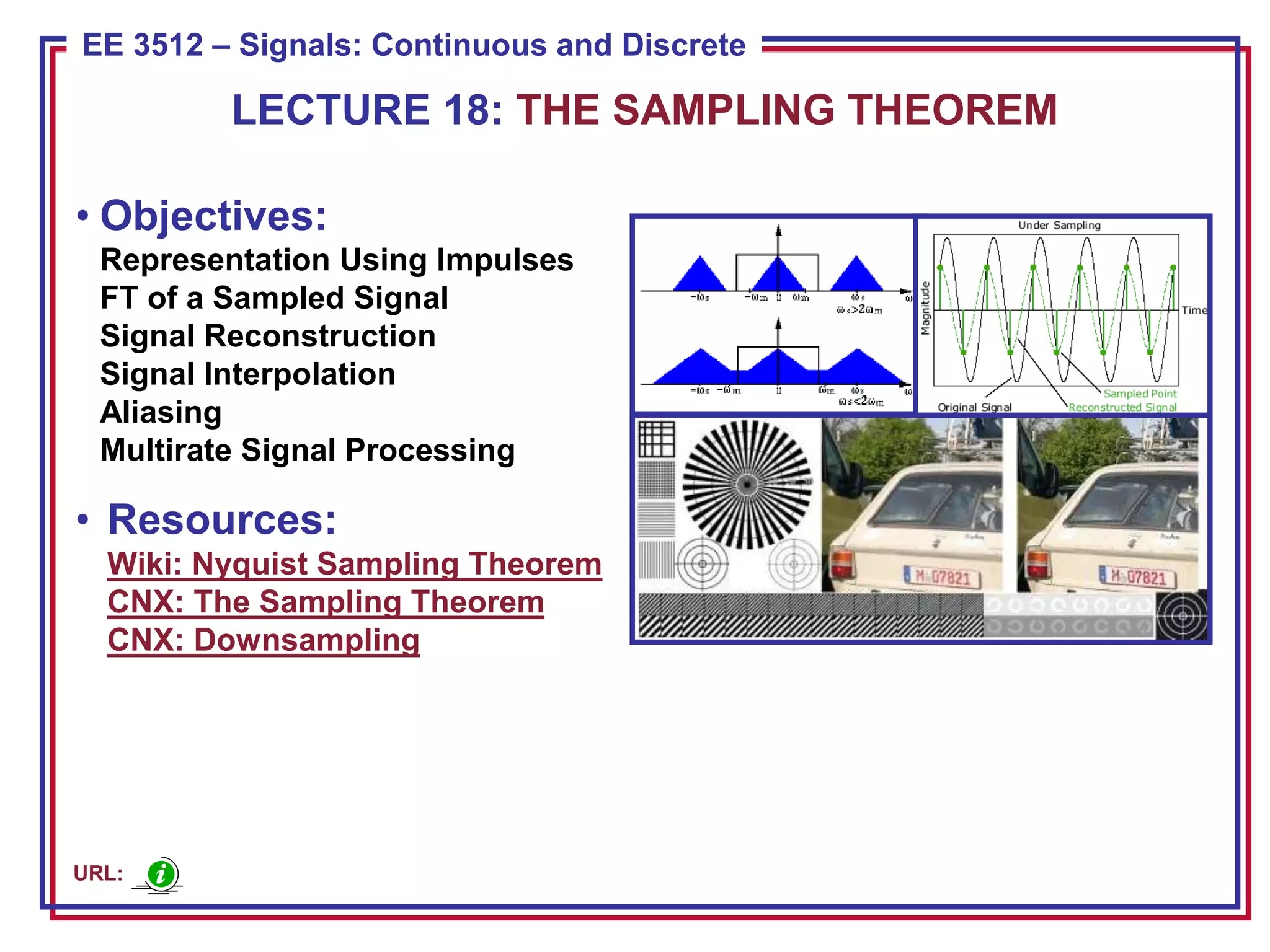
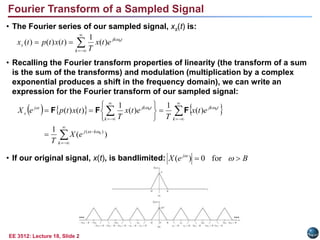
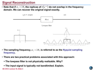
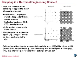
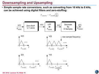
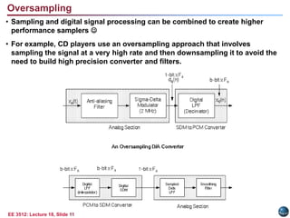
ECE 8443 – Pattern Recognition
EE 3512 – Signals: Continuous and Discrete
• Objectives:
Representation Using Impulses
FT of a Sampled Signal
Signal Reconstruction
Signal Interpolation
Aliasing
Multirate Signal Processing
• Resources:
Wiki: Nyquist Sampling Theorem
CNX: The Sampling Theorem
CNX: Downsampling
LECTURE 18: THE SAMPLING THEOREM
URL:
EE 3512: Lecture 18, Slide 1
Representation of a CT Signal Using Impulse Functions
• The goal of this lecture is to convince you that bandlimited CT signals, when
sampled properly, can be represented as discrete-time signals with NO loss of
information. This remarkable result is known as the Sampling Theorem.
• Recall our expression for a pulse train:
• A sampled version of a CT signal, x(t), is:
This is known as idealized sampling.
• We can derive the complex Fourier series of a pulse train:
   













n
n
s nT
t
nT
x
nT
t
t
x
t
p
t
x
t
x 
 )
(
)
(
)
(
)
(
)
(






n
nT
t
t
p )
(
)
( 
 























k
t
jk
t
t
jk
T
T
t
jk
T
T
t
jk
k
k
t
jk
k
e
T
t
p
T
e
T
dt
e
t
T
dt
e
t
p
T
c
T
e
c
t
p
0
0
0
0
0
1
)
(
1
1
)
(
1
)
(
1
/
2
where
)
(
0
2
/
2
/
2
/
2
/
0








t
x(t)
-2T -T 0 T 2T
…
…
EE 3512: Lecture 18, Slide 2
• The Fourier series of our sampled signal, xs(t) is:
• Recalling the Fourier transform properties of linearity (the transform of a sum
is the sum of the transforms) and modulation (multiplication by a complex
exponential produces a shift in the frequency domain), we can write an
expression for the Fourier transform of our sampled signal:
• If our original signal, x(t), is bandlimited:
Fourier Transform of a Sampled Signal






k
t
jk
s e
t
x
T
t
x
t
p
t
x 0
)
(
1
)
(
)
(
)
( 
     























k
k
j
k
t
jk
k
t
jk
j
s
e
X
T
e
t
x
T
e
t
x
T
t
x
t
p
e
X
)
(
1
)
(
1
)
(
1
)
(
)
(
)
( 0
0
0





F
F
F
B
e
X j

 

for
0
)
(
EE 3512: Lecture 18, Slide 3
Signal Reconstruction
• Note that if , the replicas of do not overlap in the frequency
domain. We can recover the original signal exactly.
B
s 2

  

j
e
X
B
s 2


• The sampling frequency, , is referred to as the Nyquist sampling
frequency.
• There are two practical problems associated with this approach:
 The lowpass filter is not physically realizable. Why?
 The input signal is typically not bandlimited. Explain.
EE 3512: Lecture 18, Slide 4
Signal Interpolation
• The frequency response of the lowpass, or interpolation, filter is:
• The impulse response of this filter is given by:
• The output of the interpolating filter is given by the convolution integral:
• Using the sifting property of the impulse:


 



elsewhere
,
0
,
)
(
B
B
T
e
H j 

 
 






 t
(Bt/πB
BT
Bt
Bt
BT
t
h sinc
/
/
sin
)
(




     
   
 
 
 








































n
n
n
s
s
d
t
h
nT
t
nT
x
d
t
h
nT
t
nT
x
d
t
h
nT
t
nT
x
d
t
h
x
t
x
t
h
t
y












)
(
)
(
)
(
)
(
)
(
)
(
)
(
*
)
(
)
(
   
 

 














n
n
nT
t
h
nT
x
d
t
h
nT
t
nT
x
t
y
)
(
)
(
)
( 


EE 3512: Lecture 18, Slide 5
Signal Interpolation (Cont.)
• Inserting our expression for the
impulse response:
• This has an interesting graphical
interpretation shown to the right.
• This formula describes a way to
perfectly reconstruct a signal from
its samples.
• Applications include digital to
analog conversion, and changing
the sample frequency (or period)
from one value to another, a process
we call resampling (up/down).
• But remember that this is still a
noncausal system so in practical
systems we must approximate this
equation. Such implementations
are studied more extensively in an
introductory DSP class.






n
nT
t
B
nT
x
BT
t
y ))
(
(
sinc
)
(
)
(


EE 3512: Lecture 18, Slide 6
Aliasing
• Recall that a time-limited signal cannot be bandlimited. Since all signals are
more or less time-limited, they cannot be bandlimited. Therefore, we must
lowpass filter most signals before sampling. This is called an anti-aliasing
filter and are typically built into an analog to digital (A/D) converter.
• If the signal is not bandlimited distortion will occur when the signal is
sampled. We refer to this distortion as aliasing:
• How was the sample frequency for CDs and MP3s selected?
EE 3512: Lecture 18, Slide 7
Sampling of Narrowband Signals
• What is the lowest sample frequency
we can use for the narrowband signal
shown to the right?
• Recalling that the process of
sampling shifts the spectrum of the
signal, we can derive a generalization
of the Sampling Theorem in terms of
the physical bandwidth occupied by
the signal.
• A general guideline is , where B = B2 – B1.
• A more rigorous equation depends on B1 and B2:
• Sampling can also be thought of as a modulation operation, since it shifts a
signal’s spectrum in frequency.
B
f
B s 4
2 

  )
to
equal
or
than
greater
integer
greatest
(
2
/
)
(
and
2
/
where
2
2
1
r
r
r
B
B
f
B
B
f
r
r
r
B
f
c
c
s









EE 3512: Lecture 18, Slide 8
Undersampling and Oversampling of a Signal
EE 3512: Lecture 18, Slide 9
Sampling is a Universal Engineering Concept
• Note that the concept of
sampling is applied to many
electronic systems:
 electronics: CD players,
switched capacitor filters,
power systems
 biological systems: EKG,
EEG, blood pressure
 information systems: the
stock market.
• Sampling can be applied in
space (e.g., images) as well
as time, as shown to the
right.
• Full-motion video signals are sampled spatially (e.g., 1280x1024 pixels at 100
pixels/inch) , temporally (e.g., 30 frames/sec), and with respect to color (e.g.,
RGB at 8 bits/color). How were these settings arrived at?
EE 3512: Lecture 18, Slide 10
Downsampling and Upsampling
• Simple sample rate conversions, such as converting from 16 kHz to 8 kHz,
can be achieved using digital filters and zero-stuffing:
EE 3512: Lecture 18, Slide 11
Oversampling
• Sampling and digital signal processing can be combined to create higher
performance samplers 
• For example, CD players use an oversampling approach that involves
sampling the signal at a very high rate and then downsampling it to avoid the
need to build high precision converter and filters.
EE 3512: Lecture 18, Slide 12
Summary
• Introduced the Sampling Theorem and discussed the conditions under which
analog signals can be represented as discrete-time signals with no loss of
information.
• Discussed the spectrum of a discrete-time signal.
• Demonstrated how to reconstruct and interpolate a signal using sinc
functions that are a consequence of the Sampling Theorem.
• Introduced a variety of applications involving sampling including
downsampling and oversampling.

Lecture 18 (5)

  • 1.
    ECE 8443 –Pattern Recognition EE 3512 – Signals: Continuous and Discrete • Objectives: Representation Using Impulses FT of a Sampled Signal Signal Reconstruction Signal Interpolation Aliasing Multirate Signal Processing • Resources: Wiki: Nyquist Sampling Theorem CNX: The Sampling Theorem CNX: Downsampling LECTURE 18: THE SAMPLING THEOREM URL:
  • 2.
    EE 3512: Lecture18, Slide 1 Representation of a CT Signal Using Impulse Functions • The goal of this lecture is to convince you that bandlimited CT signals, when sampled properly, can be represented as discrete-time signals with NO loss of information. This remarkable result is known as the Sampling Theorem. • Recall our expression for a pulse train: • A sampled version of a CT signal, x(t), is: This is known as idealized sampling. • We can derive the complex Fourier series of a pulse train:                  n n s nT t nT x nT t t x t p t x t x   ) ( ) ( ) ( ) ( ) (       n nT t t p ) ( ) (                           k t jk t t jk T T t jk T T t jk k k t jk k e T t p T e T dt e t T dt e t p T c T e c t p 0 0 0 0 0 1 ) ( 1 1 ) ( 1 ) ( 1 / 2 where ) ( 0 2 / 2 / 2 / 2 / 0         t x(t) -2T -T 0 T 2T … …
  • 3.
    EE 3512: Lecture18, Slide 2 • The Fourier series of our sampled signal, xs(t) is: • Recalling the Fourier transform properties of linearity (the transform of a sum is the sum of the transforms) and modulation (multiplication by a complex exponential produces a shift in the frequency domain), we can write an expression for the Fourier transform of our sampled signal: • If our original signal, x(t), is bandlimited: Fourier Transform of a Sampled Signal       k t jk s e t x T t x t p t x 0 ) ( 1 ) ( ) ( ) (                               k k j k t jk k t jk j s e X T e t x T e t x T t x t p e X ) ( 1 ) ( 1 ) ( 1 ) ( ) ( ) ( 0 0 0      F F F B e X j     for 0 ) (
  • 4.
    EE 3512: Lecture18, Slide 3 Signal Reconstruction • Note that if , the replicas of do not overlap in the frequency domain. We can recover the original signal exactly. B s 2      j e X B s 2   • The sampling frequency, , is referred to as the Nyquist sampling frequency. • There are two practical problems associated with this approach:  The lowpass filter is not physically realizable. Why?  The input signal is typically not bandlimited. Explain.
  • 5.
    EE 3512: Lecture18, Slide 4 Signal Interpolation • The frequency response of the lowpass, or interpolation, filter is: • The impulse response of this filter is given by: • The output of the interpolating filter is given by the convolution integral: • Using the sifting property of the impulse:        elsewhere , 0 , ) ( B B T e H j              t (Bt/πB BT Bt Bt BT t h sinc / / sin ) (                                                             n n n s s d t h nT t nT x d t h nT t nT x d t h nT t nT x d t h x t x t h t y             ) ( ) ( ) ( ) ( ) ( ) ( ) ( * ) ( ) (                        n n nT t h nT x d t h nT t nT x t y ) ( ) ( ) (   
  • 6.
    EE 3512: Lecture18, Slide 5 Signal Interpolation (Cont.) • Inserting our expression for the impulse response: • This has an interesting graphical interpretation shown to the right. • This formula describes a way to perfectly reconstruct a signal from its samples. • Applications include digital to analog conversion, and changing the sample frequency (or period) from one value to another, a process we call resampling (up/down). • But remember that this is still a noncausal system so in practical systems we must approximate this equation. Such implementations are studied more extensively in an introductory DSP class.       n nT t B nT x BT t y )) ( ( sinc ) ( ) (  
  • 7.
    EE 3512: Lecture18, Slide 6 Aliasing • Recall that a time-limited signal cannot be bandlimited. Since all signals are more or less time-limited, they cannot be bandlimited. Therefore, we must lowpass filter most signals before sampling. This is called an anti-aliasing filter and are typically built into an analog to digital (A/D) converter. • If the signal is not bandlimited distortion will occur when the signal is sampled. We refer to this distortion as aliasing: • How was the sample frequency for CDs and MP3s selected?
  • 8.
    EE 3512: Lecture18, Slide 7 Sampling of Narrowband Signals • What is the lowest sample frequency we can use for the narrowband signal shown to the right? • Recalling that the process of sampling shifts the spectrum of the signal, we can derive a generalization of the Sampling Theorem in terms of the physical bandwidth occupied by the signal. • A general guideline is , where B = B2 – B1. • A more rigorous equation depends on B1 and B2: • Sampling can also be thought of as a modulation operation, since it shifts a signal’s spectrum in frequency. B f B s 4 2     ) to equal or than greater integer greatest ( 2 / ) ( and 2 / where 2 2 1 r r r B B f B B f r r r B f c c s         
  • 9.
    EE 3512: Lecture18, Slide 8 Undersampling and Oversampling of a Signal
  • 10.
    EE 3512: Lecture18, Slide 9 Sampling is a Universal Engineering Concept • Note that the concept of sampling is applied to many electronic systems:  electronics: CD players, switched capacitor filters, power systems  biological systems: EKG, EEG, blood pressure  information systems: the stock market. • Sampling can be applied in space (e.g., images) as well as time, as shown to the right. • Full-motion video signals are sampled spatially (e.g., 1280x1024 pixels at 100 pixels/inch) , temporally (e.g., 30 frames/sec), and with respect to color (e.g., RGB at 8 bits/color). How were these settings arrived at?
  • 11.
    EE 3512: Lecture18, Slide 10 Downsampling and Upsampling • Simple sample rate conversions, such as converting from 16 kHz to 8 kHz, can be achieved using digital filters and zero-stuffing:
  • 12.
    EE 3512: Lecture18, Slide 11 Oversampling • Sampling and digital signal processing can be combined to create higher performance samplers  • For example, CD players use an oversampling approach that involves sampling the signal at a very high rate and then downsampling it to avoid the need to build high precision converter and filters.
  • 13.
    EE 3512: Lecture18, Slide 12 Summary • Introduced the Sampling Theorem and discussed the conditions under which analog signals can be represented as discrete-time signals with no loss of information. • Discussed the spectrum of a discrete-time signal. • Demonstrated how to reconstruct and interpolate a signal using sinc functions that are a consequence of the Sampling Theorem. • Introduced a variety of applications involving sampling including downsampling and oversampling.

Editor's Notes

  • #2 MS Equation 3.0 was used with settings of: 18, 12, 8, 18, 12.
  • #3 ]i=k,