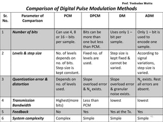
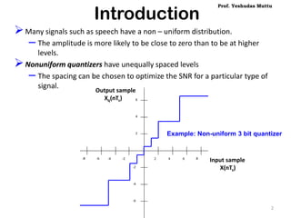
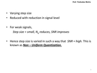
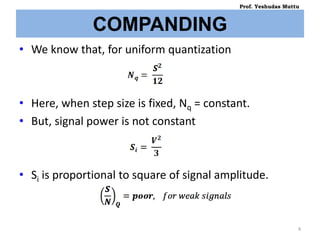
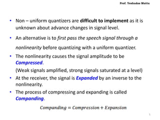
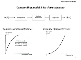
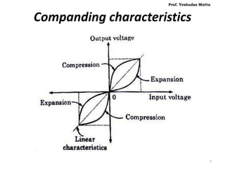
The document discusses non-uniform quantization and its advantages for signals with a non-uniform distribution, emphasizing the concept of varying step sizes to optimize signal-to-noise ratio (SNR). It introduces companding as a process to compress signals before quantization and discusses different companding laws (μ-law and A-law) used in telecommunication systems. Additionally, it covers various pulse code modulation (PCM) techniques, including differential PCM and delta modulation, highlighting their advantages and disadvantages in terms of complexity and bandwidth requirements.

1. NON – UNIFORM
QUANTIZATION
Prof. Yeshudas A. Muttu
Assistant Professor
Don Bosco College of Engineering, Fatorda – Goa
1

2. Introduction
Many signals such as speech have a non – uniform distribution.
– The amplitude is more likely to be close to zero than to be at higher
levels.
Nonuniform quantizers have unequally spaced levels
– The spacing can be chosen to optimize the SNR for a particular type of
signal.
2 4 6 8
2
4
6
-2
-4
-6
Input sample
X(nTs)
Output sample
Xq(nTs)
-2-4-6-8
Example: Non-uniform 3 bit quantizer
Prof. Yeshudas Muttu
2

3. • Varying step size
• Reduced with reduction in signal level
• For weak signals,
Step size = small, Nq reduces, SNR improves
• Hence step size is varied in such a way that SNR = high. This is
known as Non – Uniform Quantization.
Prof. Yeshudas Muttu
3

4. COMPANDING
• We know that, for uniform quantization
• Here, when step size is fixed, Nq = constant.
• But, signal power is not constant
• Si is proportional to square of signal amplitude.
Prof. Yeshudas Muttu
4

5. • Non – uniform quantizers are difficult to implement as it is
unknown about advance changes in signal level.
• An alternative is to first pass the speech signal through a
nonlinearity before quantizing with a uniform quantizer.
• The nonlinearity causes the signal amplitude to be
Compressed.
(Weak signals amplified, strong signals saturated at a level)
• At the receiver, the signal is Expanded by an inverse to the
nonlinearity.
• The process of compressing and expanding is called
Companding.
Prof. Yeshudas Muttu
5

6. Companding model & its characteristics
m(t)
Compressor Characteristics Expander Characteristics
Compressor
Uniform
Quantizer Expander
Prof. Yeshudas Muttu
6

7. Companding characteristics
Prof. Yeshudas Muttu
7

8. Types of Companding
• Ideally, we need linear characteristics for small
amplitude signals & a logarithmic characteristic.
• Practically, this achieved by
1. - law Companding
2. A- law Companding
Prof. Yeshudas Muttu
8

9. - law Companding
• Here, compressor characteristics is continuous.
• Approx. Linear, for smaller values of input & logarithmic for higher
input levels.
• - law characteristic is mathematically given as :
• Where y = output & x = input to the compressor
• = normalised input w.r.t. the maximum value, z(x) = y/xmax.
• Practically used value of is 255.
Prof. Yeshudas Muttu
9

10. • If = 0, the characteristics correspond to uniform
quantization (fig a).
• law companding is used for Speech and music signals.
• Also used for PCM telephone systems in U.S., Canada & Japan.
• Fig(b) shows variation of (SNR)q w.r.t. Signal level, with &
without companding.
• With companding, SNR is almost constant at all signal levels.
• It has mid tread at the origin. Hence it contains zero value
Prof. Yeshudas Muttu
10

11. A - law Companding
• Here, compressor characteristic is piece – wise made up of
linear segment for low input levels & logarithmic segment for
high level inputs.
• Used for PCM telephone systems elsewhere. (European
standard).
Prof. Yeshudas Muttu
11

12. • For A = 1, linear characteristics  uniform quantization.
• Practically, A = 87.56 is used since it provides better non –
linearity for high level inputs.
• A – law has midrise at the origin. Hence it contains non – zero
value.
Prof. Yeshudas Muttu
12

13. PULSE CODE MODULATION
Prof. Yeshudas Muttu
13

14. Prof. Yeshudas Muttu
14

15. Electrical representation
Prof. Yeshudas Muttu
15

16. Block diagram for PCM
• A/D converter accepts an analog signal & replaces it
with respective code symbols.
• Each symbol consists of train of pulses.
• Digitally encoded signal is transmitted.
Prof. Yeshudas Muttu
16

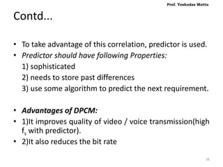
17. Contd...
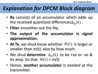
• At the Receiver,
• Separation of noise due to channel.
• Done by Quantization.(Re quantization)
• Simple decision, For each Pulse duration, pulse Rxed or not.
• If quantized signal was sent in place of digitally encoded signal:
• At rx, it wud hav to deal with all the levels of quantization.
• [Advantage : Reliable since we send digitally encoded signal rather than
jus quantized signal]
• Quantizer sends its decision to the decoder(D/A) in the form of
regenerated pulse train
• Output of decoder is quantized multilevel sample pulses.
• This is then filtered to obtain msg signal back.
Prof. Yeshudas Muttu
17

18. Advantages of PCM system:
1. Very high noise immunity.
2. Due to digital nature, repeaters can be placed between
Transmitter & Receiver which is not possible in analog
systems.
3. Due to digital nature, it is possible to store PCM signal.
4. It is possible to use various coding techniques so that
only desired person can decode the received signal.
Disadvantages of PCM system:
1. Encoding, decoding & quantizer circuits are complex.
2. Requires large Bandwidth as compared to other
systems.
Prof. Yeshudas Muttu
18

19. Applications of PCM
1. In telephony (optical fibres)
2. In space communication
– Space craft transmits signals to earth
– Transmitted signal power is very low(10 to 15 W)
– Distances are huge (Km)
– Due to High noise immunity, only PCM systems
can be used in such applications.
Prof. Yeshudas Muttu
19

20. Differential PCM
Introduction:
• Here, instead of transmitting sample values,
• At each sampling time, it txs the difference between
current sample m(k) & the past sample m(k-1).
• i.e. At time k & k-1.
• If this is done, then simply by adding up these changes at
the receiver, a w/f identical to m(t) can be achieved.
• Since difference between two consecutive samples is
transmitted, modulation scheme is known as DPCM.
• This technique reduces the no. of quantization levels,
hence give rise to less no. of encoded bits .
Prof. Yeshudas Muttu
20

21. • Transmitted signal shud convey the difference
between m(t) & (t) rather than just recent
change in m(t).
• In analog systems, the difference is
precisely last change in m(t).
• In quantized systems, we add or subtract from
(t) a value, which is appropriate to bring (t)
closer to m(t).
Prof. Yeshudas Muttu
21

22. Block diagram of Differential PCM
Transmitter
Receiver
Prof. Yeshudas Muttu
22

23. Explanation for DPCM Block diagram
• Rx consists of an accumulator which adds up
the received quantized differences .
• Filter smoothes out the Nq.
• The output of the accumulator is signal
approximation.
• At Tx, we shud know whether is larger or
smaller than m(t); also by how much.
• We shud determine to be +ve or -ve &
its amp. So that = m(t).
• Hence, another accumulator is needed at the
transmitter.
Prof. Yeshudas Muttu
23

24. Explanation for DPCM Block diagram
• At each sampling tym, Tx compares &
m(t) by difference amplifier.
• The S/H cktry holds the result as at the
time between two samples.
• The quantizer generates signal with 2 purpose:
a) transmit the signal to the Rx.
b) provide it as an input to the accumulator.
• Of course, before Txn, the quantized signal will be
encoded into binary bits stream & than decoded at
the Rx
Prof. Yeshudas Muttu
24

25. Need For Predictor
• When fs = Nyquist rate, it generates excessive Nq compared to
PCM.
• Nq = reduced by increasing fs . Hence, differences from
sample to sample are smaller.
• Thus rate of producing high Nq reduces.
• But if this is done bit rate of DPCM exceed than that of PCM
• Bit rate = No. of bits per sample x Sample rate
• Hence, this situation is improved by recognizing that there is a
correlation between successive samples of signal m(t) & of
Δ(t) if signal is sampled at rate greater than Nyquist rate.
• Thus knowledge of past sample values or differences allows
us to predict with some probability to be correct.
Prof. Yeshudas Muttu
25

26. Contd...
• To take advantage of this correlation, predictor is used.
• Predictor should have following Properties:
1) sophisticated
2) needs to store past differences
3) use some algorithm to predict the next requirement.
• Advantages of DPCM:
• 1)It improves quality of video / voice transmission(high
fs with predictor).
• 2)It also reduces the bit rate
Prof. Yeshudas Muttu
26

27. Delta Modulation
• DPCM scheme in which difference signal is encoded into 1 –
bit. (i.e. To Increase or decrease the )
Linear
Delta Modulator
Prof. Yeshudas Muttu
27

28. Explanation for DM block diagram
Comparator (replaces difference amplifier & quantizer)
• m(t) & are applied to the comparator.
• m(t) > , comparator o/p = V(H)
• m(t) < , comparator o/p = V(L)
• As m(t) – passes thru’ zero, transition from V(L) to V(H)
or vice versa takes place.
Up – down counter (serves as an accumulator)
• Increments or decrements its count by 1 at each active edge
of the clock. ( let it be falling edge )
• The count direction is determined by the count direction
command.
– If V(H), it counts up.
– If V(L), it counts down.
Output of the counter is converted to
analog quantized approx. by
D/A convertor.
Prof. Yeshudas Muttu
28

29. 1 1 1 0 1 1 1 0 1 1 0 1
Prof. Yeshudas Muttu
29

30. Advantages of Delta Modulation
1. It transmits only 1 – bit per sample. Hence reducing the
transmission channel bandwidth.
2. Tx – Rx implementation is simple as compared to PCM
system.
Disadvantages of Delta Modulation
1. Poor start-up response
2. Slope Overload Distortion
3. Granular Noise/ Idle Noise
Prof. Yeshudas Muttu
30

31. 1. Poor start-up response
• Initially there is large discrepancy betn m(t) & .
Disadvantages of Delta Modulation
Prof. Yeshudas Muttu
31

32. 2. Slope Overload distortion
• m(t) exhibits slope so large that cannot cope
up with it.
• Hence error becomes more & more larger
exceeding S/2.
• This excessive error is termed as slope overload
distortion.
• Where, slope of m(t) > slope
• It can be avoided if
Prof. Yeshudas Muttu
32

33. 3. Granular Noise
• Occurs when step size is too large to small variations in the
input.
• When input is almost flat, staircase signal oscillates between
S.
• To avoid this we make step size small. But smaller step size
leads to slope overload distortion.
• To avoid these errors, Adaptive delta modulation is
employed.
Prof. Yeshudas Muttu
33

34. Adaptive Delta Modulator
• Here, step size is varied.
• During slope overload, step size is increased to match with the
m(t) signal.
Prof. Yeshudas Muttu
34

35. Explanation of ADM block diagram
• The processor has an accumulator.
• At active edge of the clock w/f, the processor generates a
step S & isolates the accumulator.
• Step size S is not fixed but is multiple of basic step S0.
Algorithm for generation of step S:
• If the direction of step at clock edge ‘k’ is same as at (k – 1)th
clock edge,
 Increase magnitude of step by S0
 Else, decrease magnitude of step by S0
• If step becomes Zero, then set S = S0 at next clk.
• e(k) = discrepancy between m(t) & i.e. Error.
Prof. Yeshudas Muttu
35

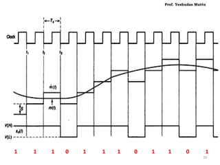
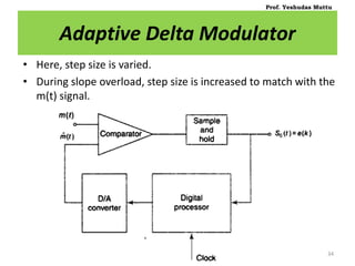
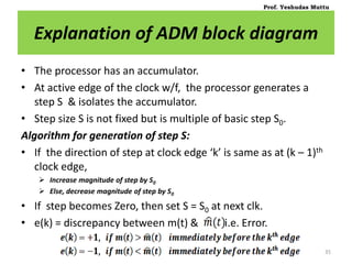
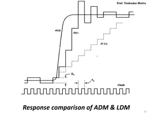
36. • Hence, at kth sampling time, step size is given by,
[ New step size ] [ old step size ] [ Some increment ]
• When m(t) > , jumps larger to match with m(t).
• But, it may take larger time for step S to decay in magnitude when
not needed.
• When m(t) = constant, oscillates about m(t) but frequency of
oscillation is half the clock freq.
• Slope overload decreases, Nq increases slightly.
• Slope overload error in reconstructed signal affects low freq. range.
• Nq introduces HF components.
• Power in speech signal is concentrated more in LF components.
• This, when passed thru’ LPF, HF components by Nq are removed.
Prof. Yeshudas Muttu
36

37. Response comparison of ADM & LDM
Prof. Yeshudas Muttu
37

38. Continuously Variable Slope DM (CVSD)
Prof. Yeshudas Muttu
Vgc
38

39. Construction
• Amplifier has variable gain.
• Its gain is a function of voltage applied at its gain – control
(Vgc) terminal.
• Assume when Vgc= 0, then amplifier gain = low.
• As Vgc increases, amplifier gain also increases.
• R – C combination serves as an integrator.
• Vc is proportional to integral of pulse signal p0(t).
• Vc is used to control the gain of the amplifier.
• Square law device ensures that whatever the polarity of the
Vc, +ve v/g will be applied to gain control terminal of the
amplifier.
Prof. Yeshudas Muttu
39

40. Assume m(t) makes small excursions such that o/p of modulator
gives alternate polarity pulses.
• These pulses when integrated gives avg. o/p = 0.
• Hence, Vgc = 0 Gain = low step size = reduces.
Consider slope overload case
• If m(t) increases + vely or – vely at a rapid rate, wont be
able to follow it.
• p0(t) is then a train of all +ve or all – ve pulses.
• Integrator averages & provides large voltage to increase the
gain of the amplifier.
• Hence step size increases whether Vgc is +ve or – ve coz of
square law device. This reduces slope overload error.
Working
Prof. Yeshudas Muttu
40

41. Comparison of Digital Pulse Modulation Methods
Sr.
No.
Parameter of
Comparison
PCM DPCM DM ADM
1 Number of bits Can use 4, 8
or 16 – bits
per sample.
Bits can be
more than
one but less
than PCM.
Uses only 1 –
bit per
sample.
Only 1 – bit is
used to
encode one
sample.
2 Levels & step size No. of levels
depends on
no. of bits.
Step size is
kept constant.
Fixed no. of
levels are
used.
Step size is
kept fixed &
cannot be
varied.
According to
signal
variations,
step size is
varied.
3 Quantization error &
distortion
Depends on
no. of levels
used.
Slope
overload error
& Nq exists.
Slope
overload error
& granular
noise exists.
Nq exists. Rest
all errors are
absent.
4 Transmission
Bandwidth
Highest(more
bits)
Less than
PCM
lowest lowest
5 Feedback No Yes Yes at the Tx. Yes
6 System complexity Complex Simple Simple Simple
Prof. Yeshudas Muttu
41

42. References
• Herbert Taub, Donald L Schilling, Goutam Saha, “Principles of
Communication systems”, 3rd edition, Mc Graw Hill.
• Tomasi, “Electronic Communication Systems”, 5th edition, Pearson.
• Sanjay Sharma, “Communication Systems (Analog & Digital)”, 4th
edition, Watson books.
Prof. Yeshudas Muttu
42