Download to read offline
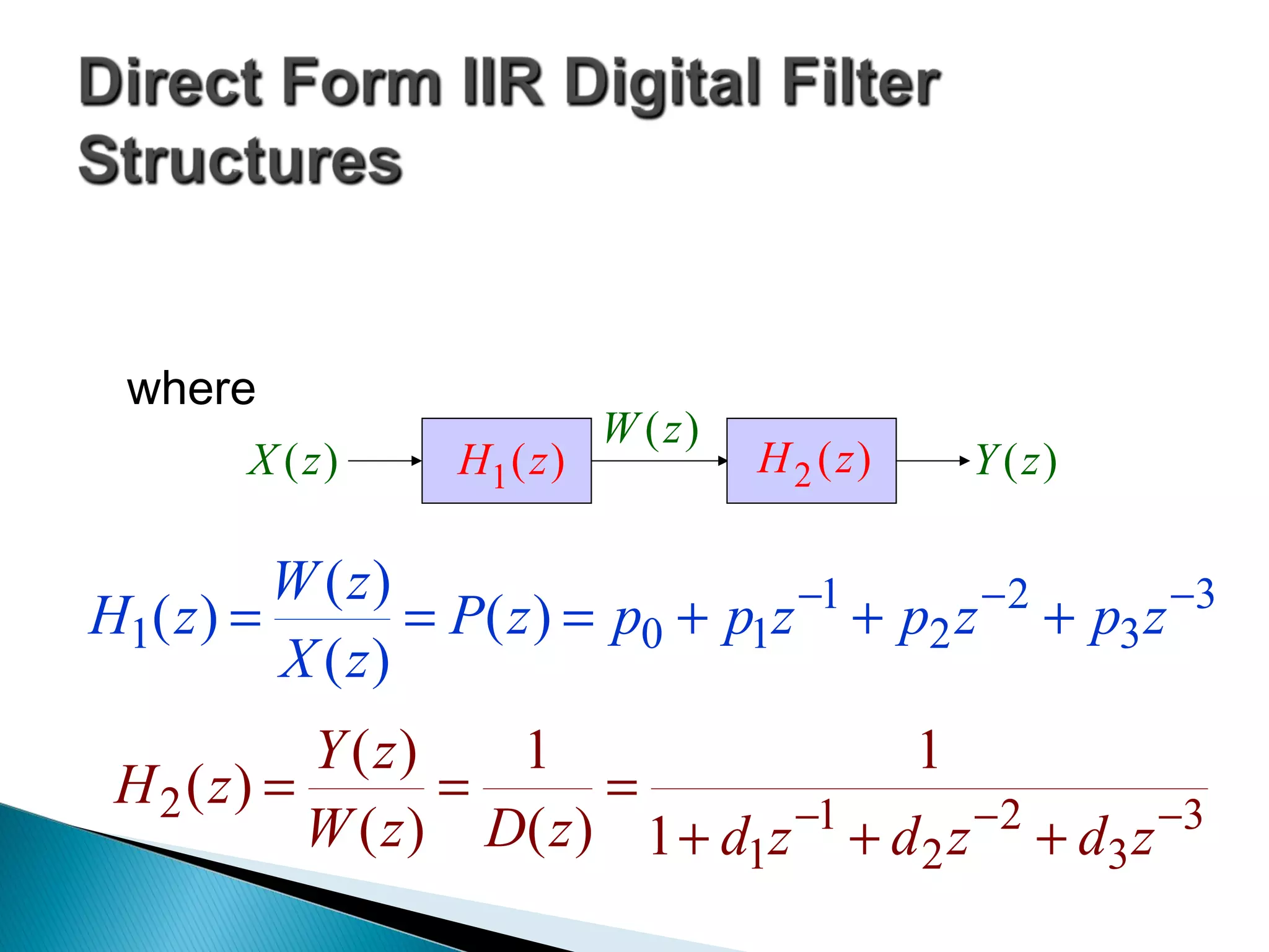
![ The filter section can be seen to be an
FIR filter and can be realized as shown below
]3[]2[]1[][][ 3210 −+−+−+= nxpnxpnxpnxpnw
)(zH1](https://image.slidesharecdn.com/structuresforfirsystems-190427205158/75/Structures-for-FIR-systems-6-2048.jpg)
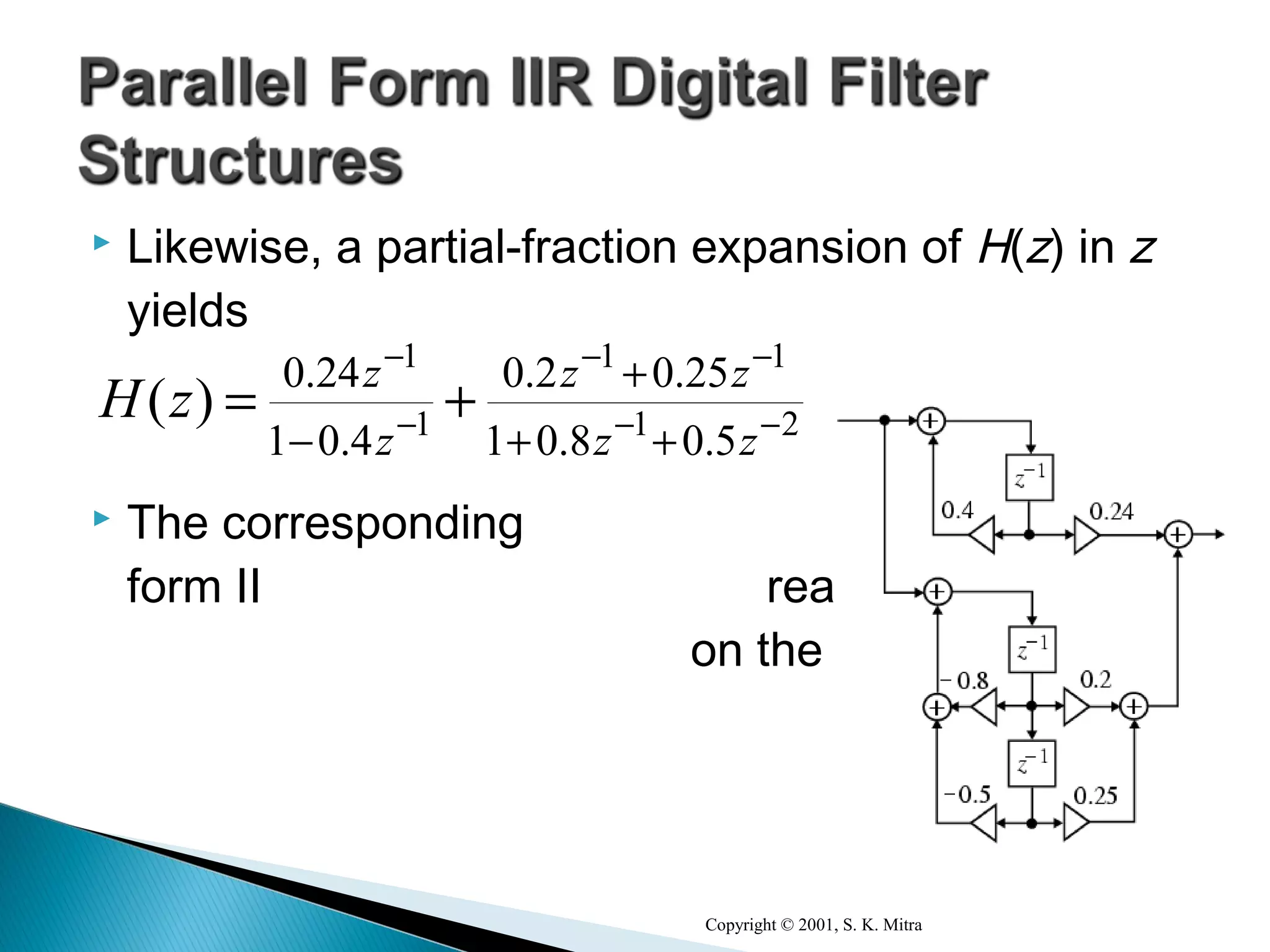
![ The time-domain representation of is
given by
Realization of follows
from the above
equation and is
shown on the right
)(zH2
][][][][][ 321 321 −−−−−−= nydnydnydnwny
)(zH2](https://image.slidesharecdn.com/structuresforfirsystems-190427205158/75/Structures-for-FIR-systems-7-2048.jpg)
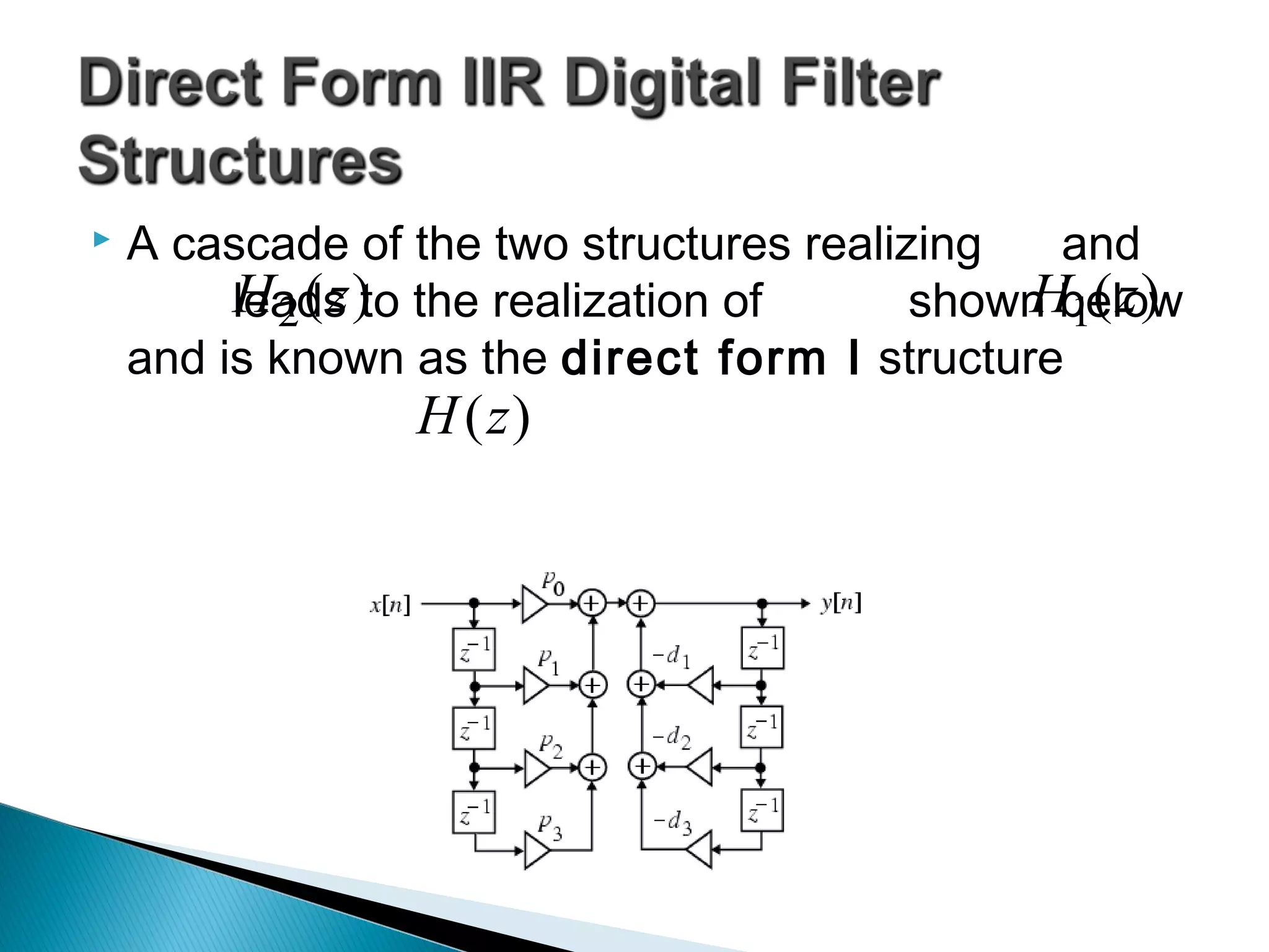
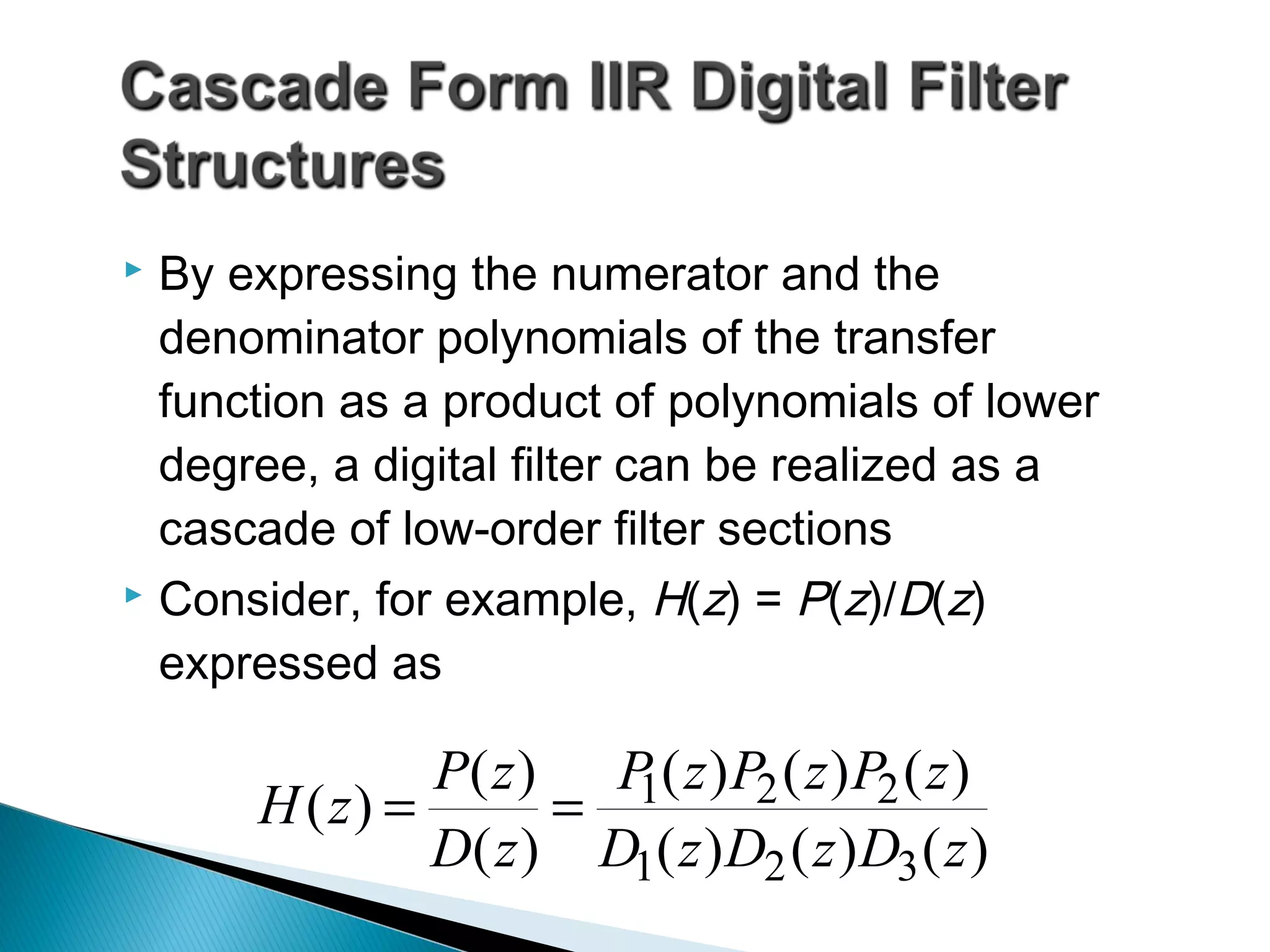

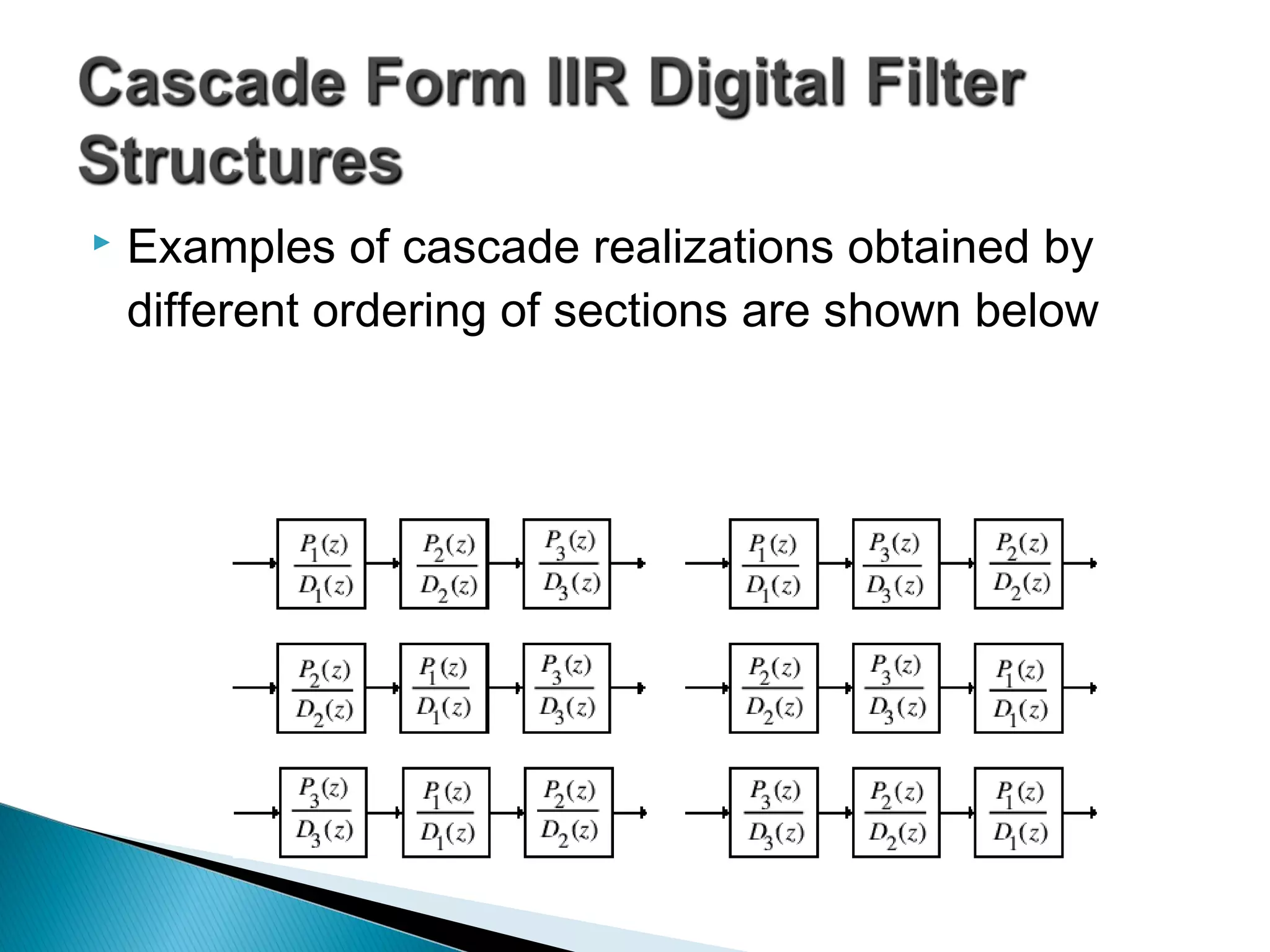

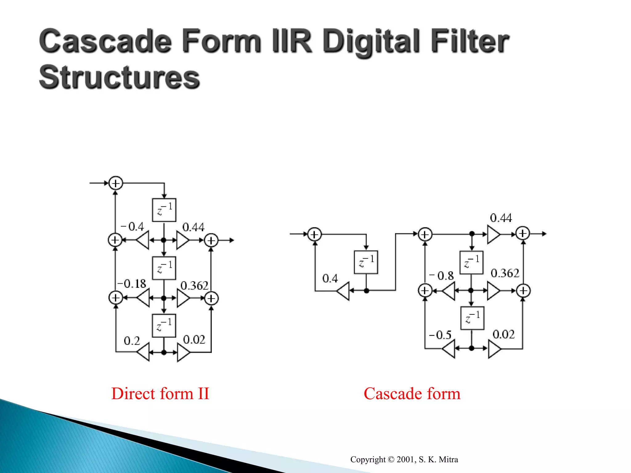
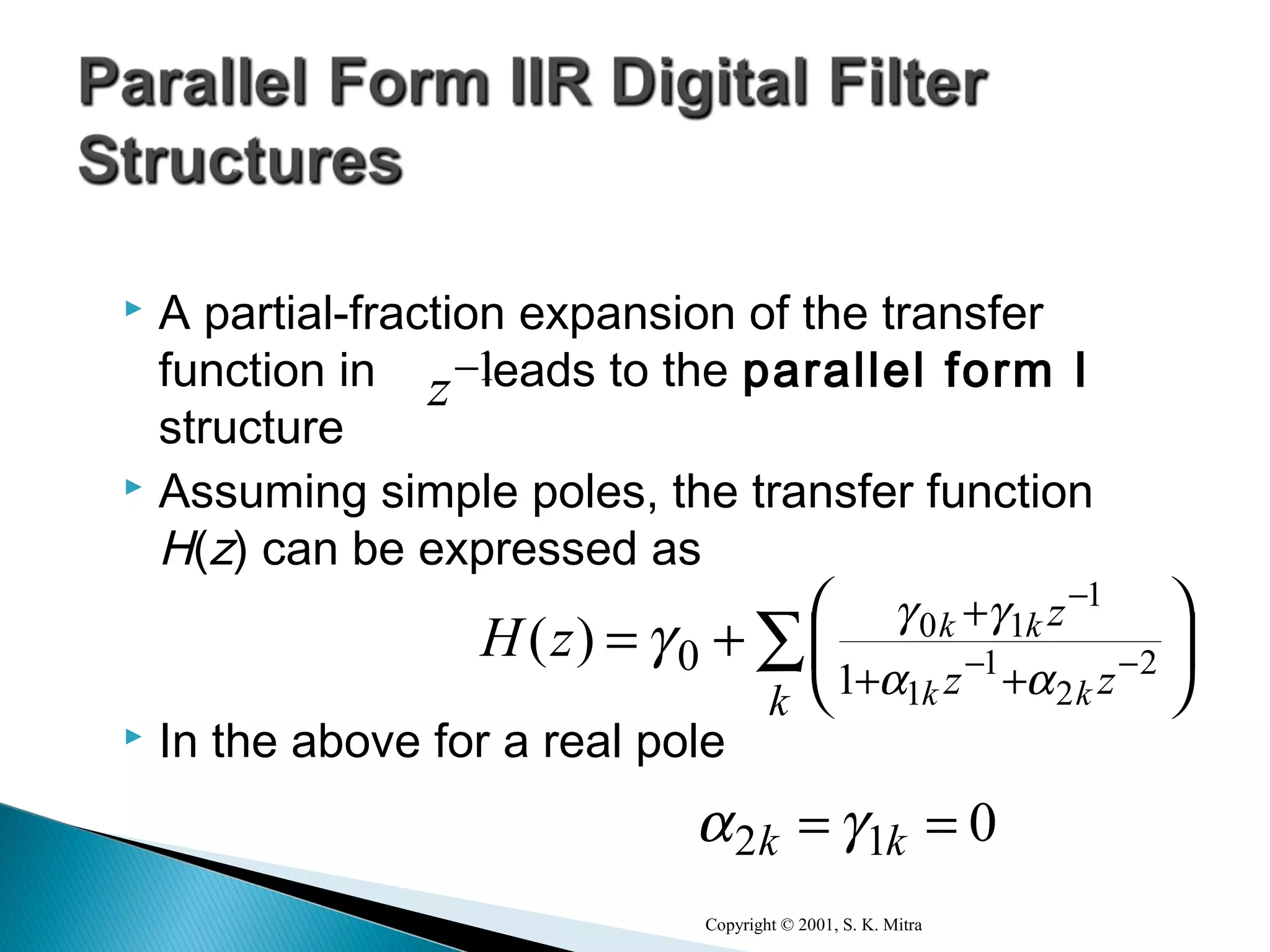
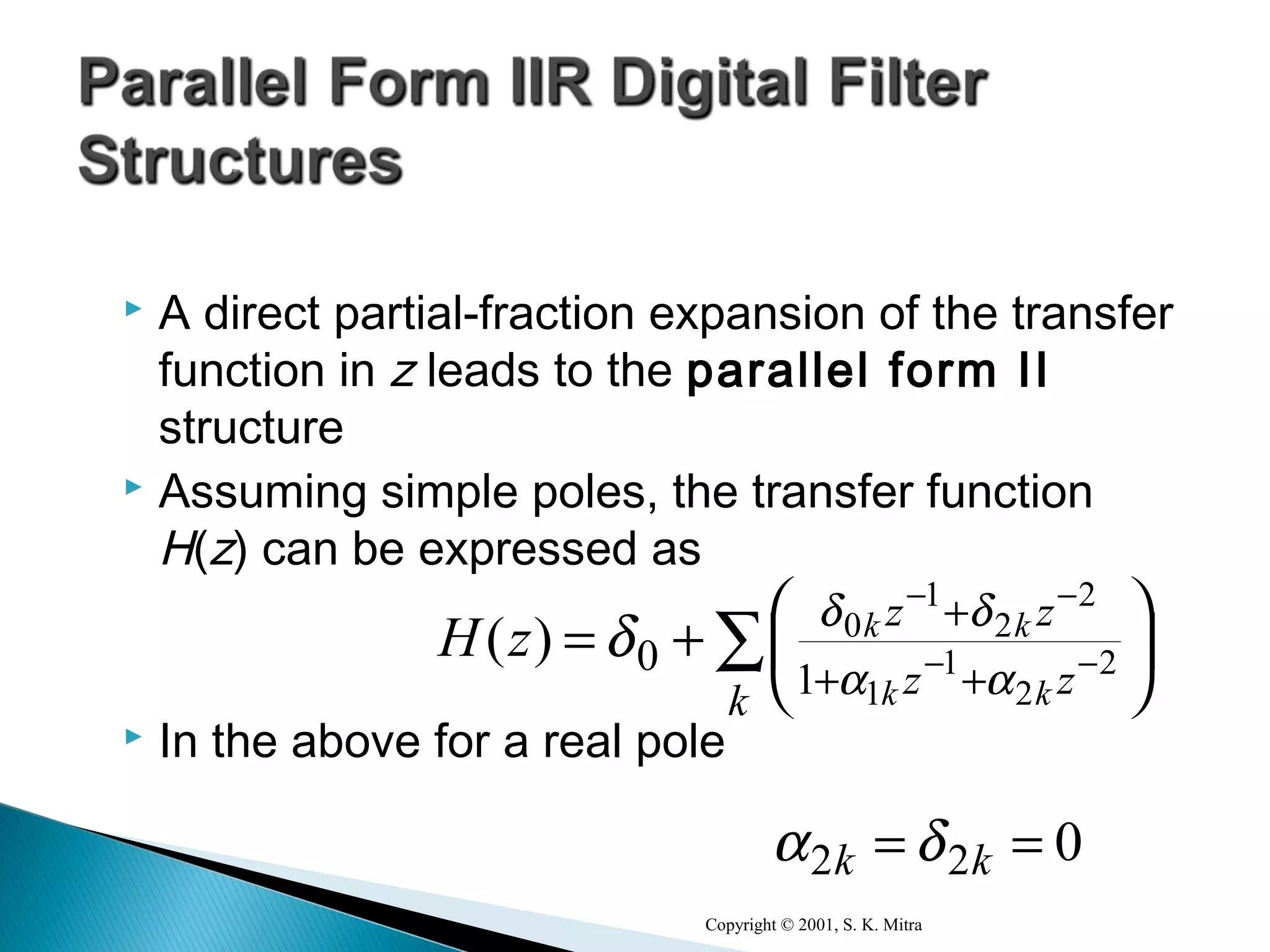
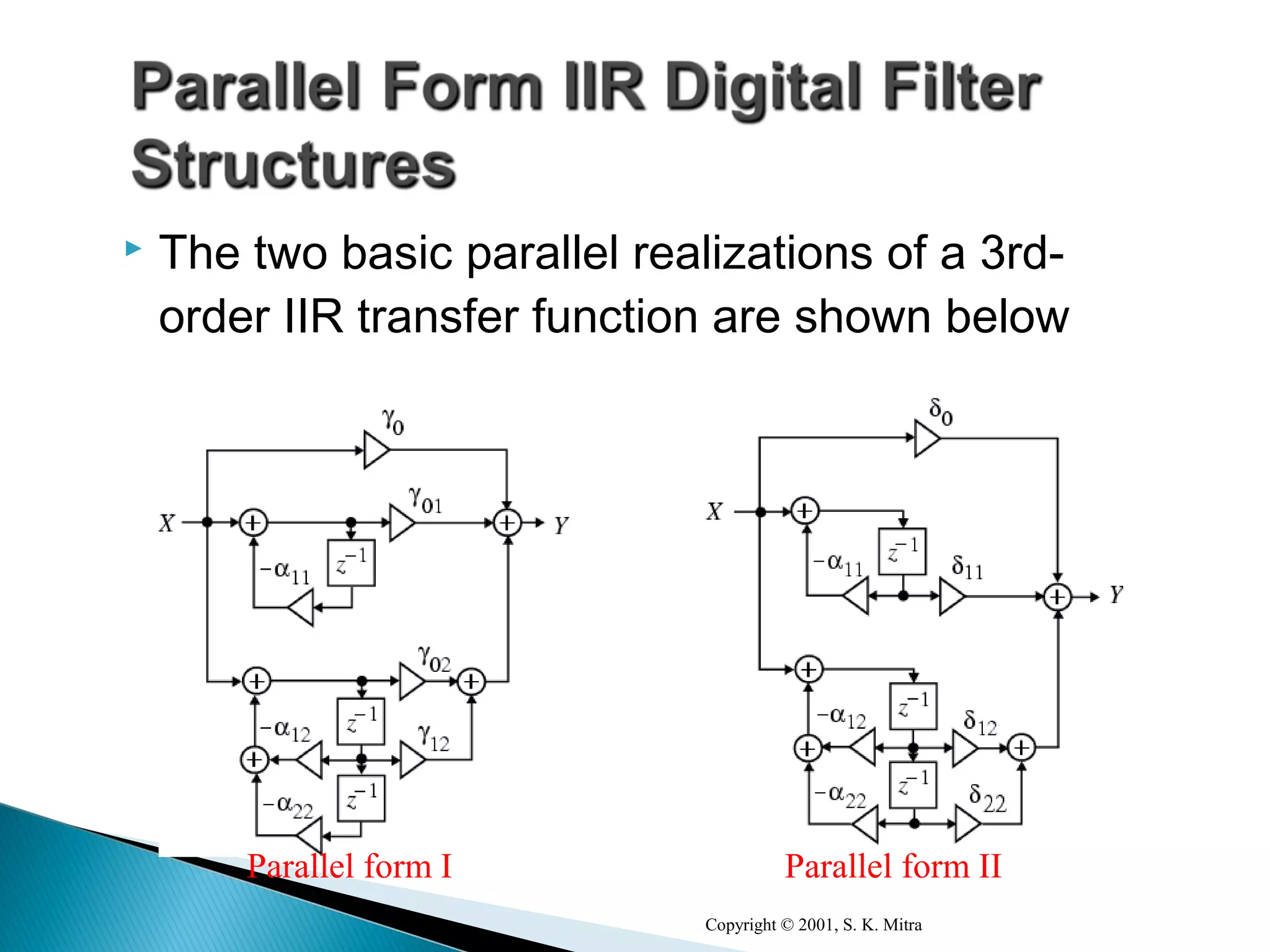
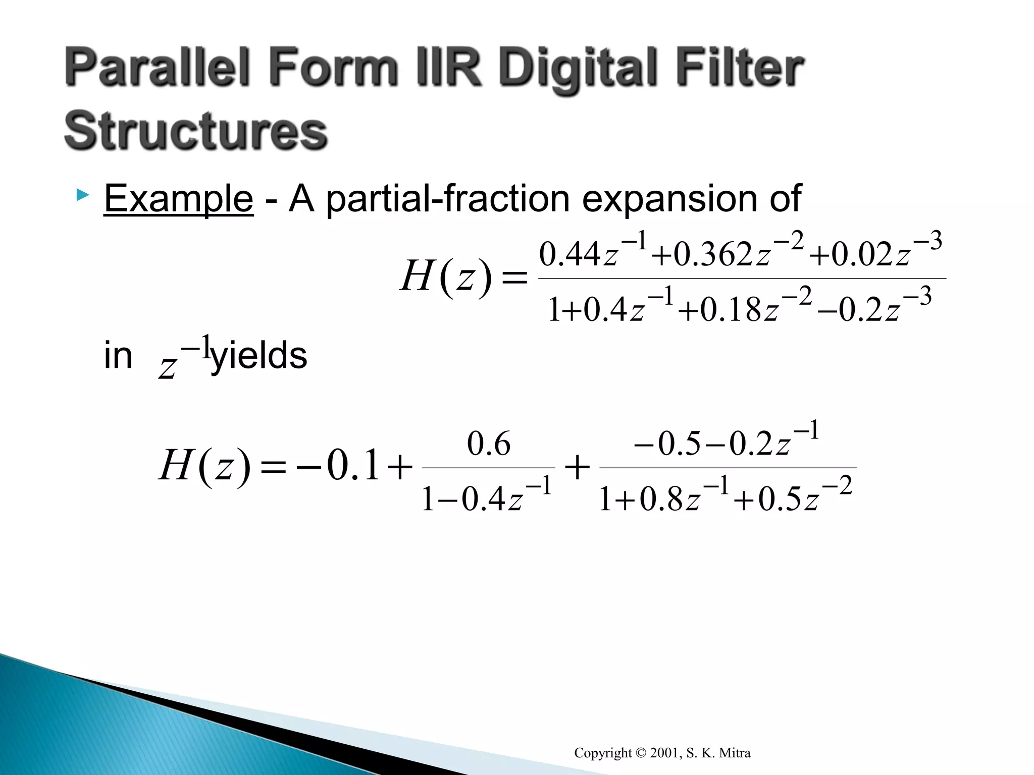
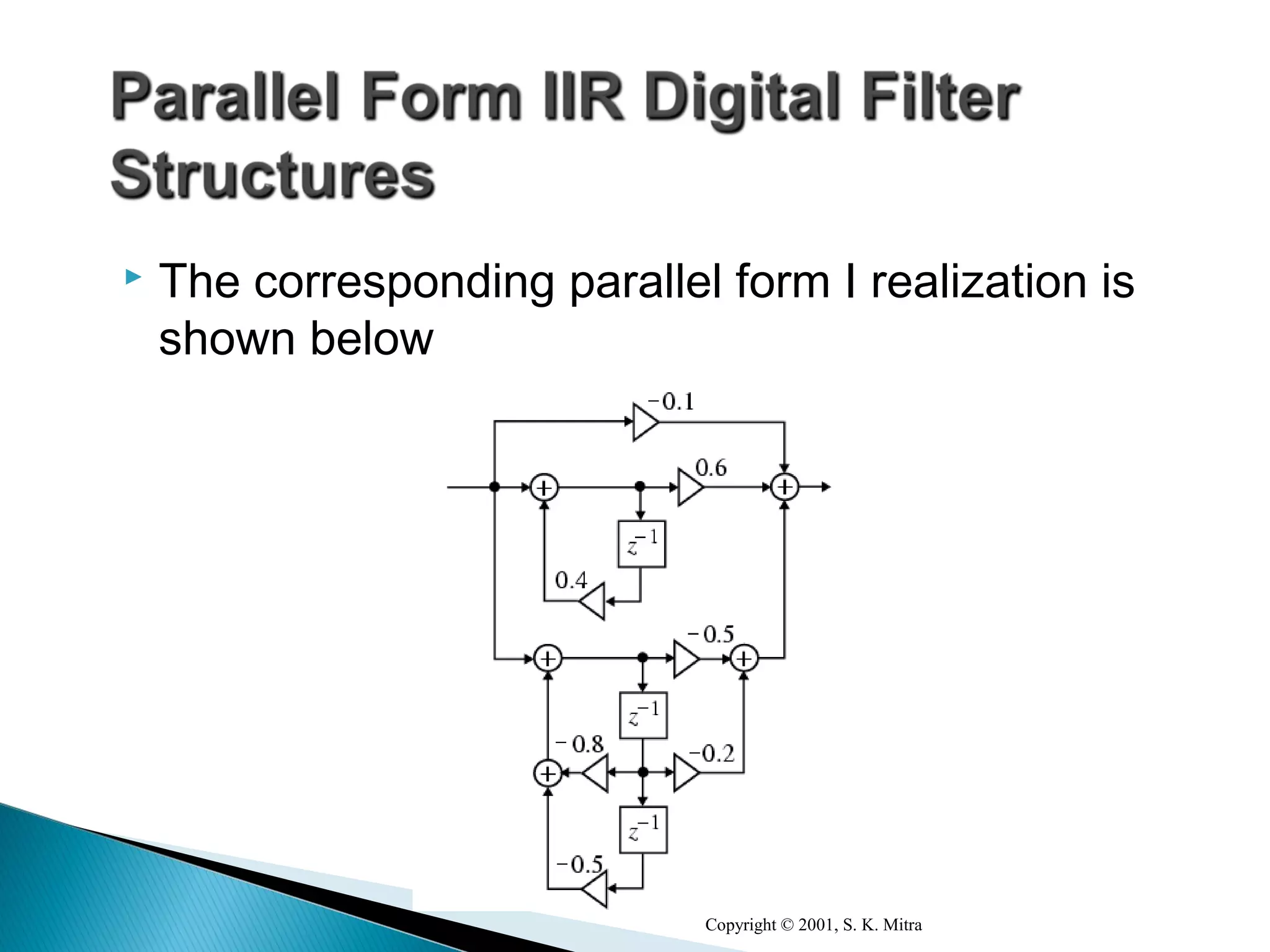


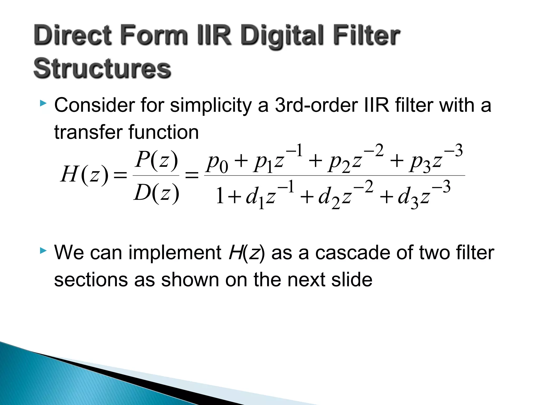
This document discusses different realization structures for causal IIR digital filters, including direct form I and II structures, cascade structures, and parallel form I and II structures. It provides examples of implementing a 3rd order IIR transfer function using each type of structure. Direct form I structures realize the coefficients directly from the transfer function. Cascade structures decompose the transfer function into lower order sections. Parallel forms use partial fraction expansions to decompose into parallel signal flows.