Download as PDF, PPTX
![Three Processes in A/D Conversion
Sampling Quanti- Binary
zation Encoding
xc(t) x[n] = xc(nT) x[n] c[n]
Sampling Quantization Binary
Period Interval codebook
T Q
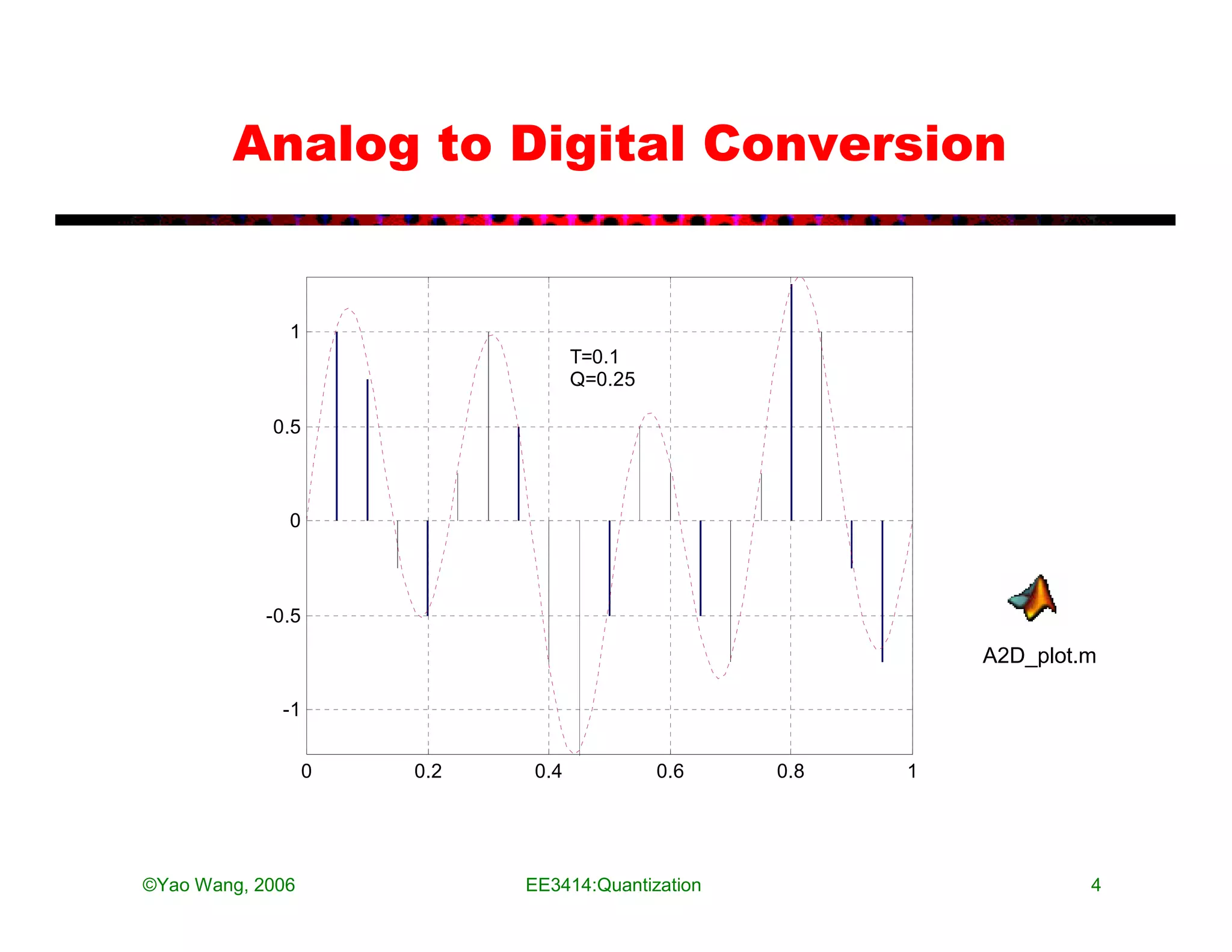
• Sampling: take samples at time nT
– T: sampling period;
– fs = 1/T: sampling frequency
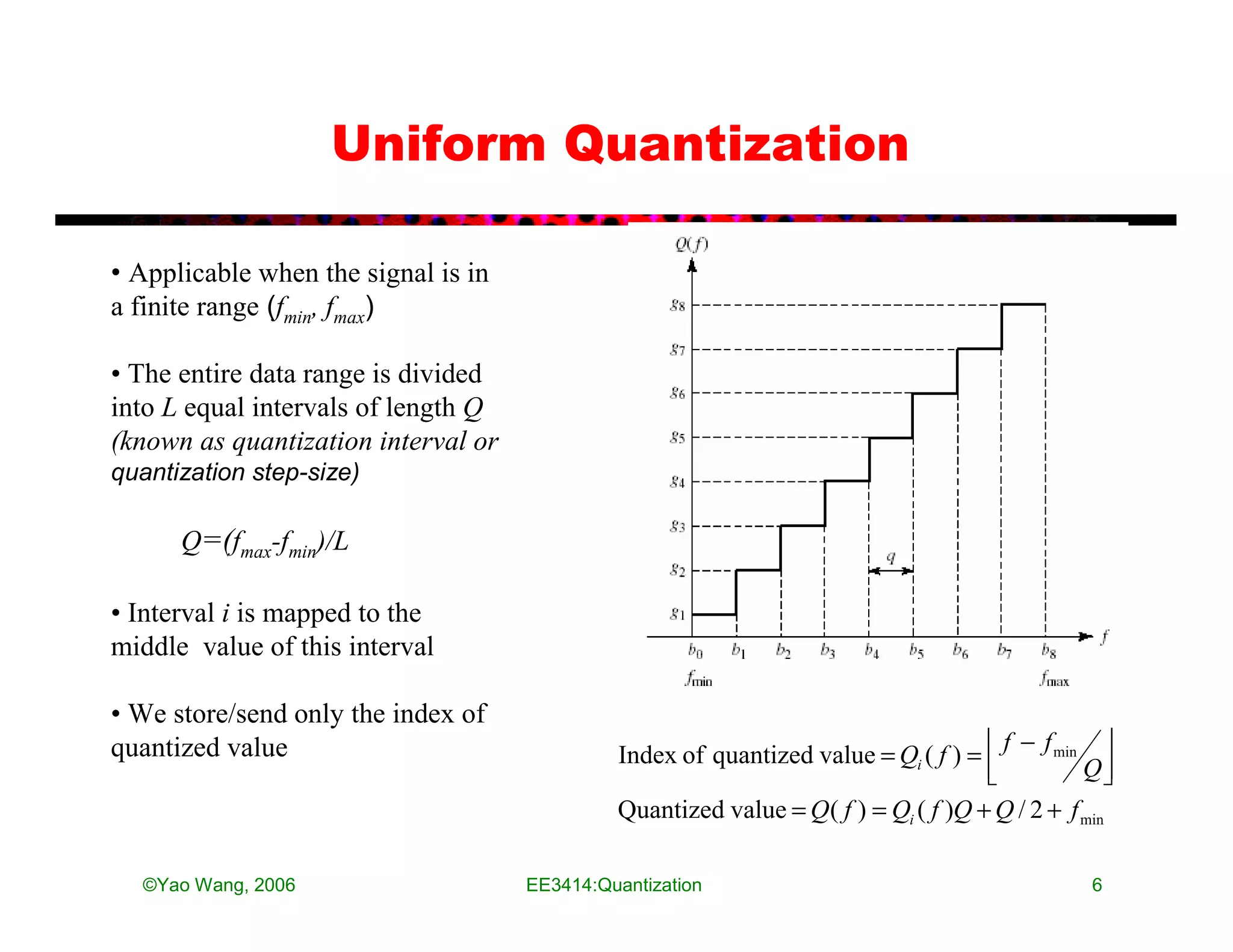
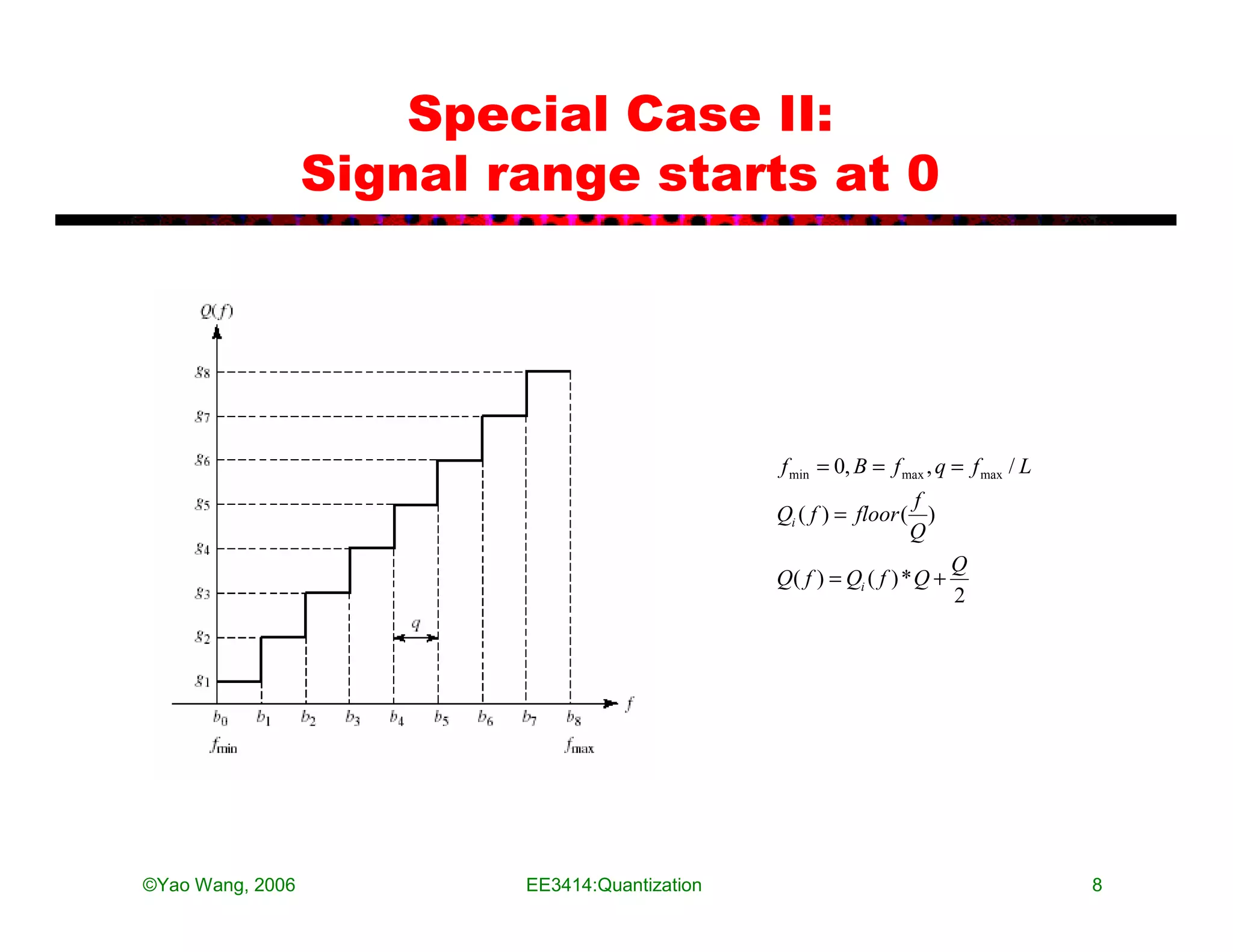
• Quantization: map amplitude values into a set of discrete values kQ
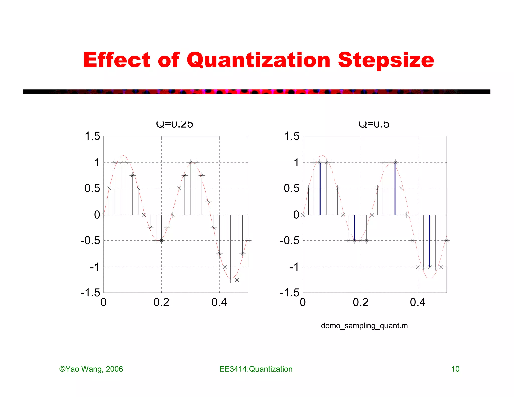
– Q: quantization interval or stepsize
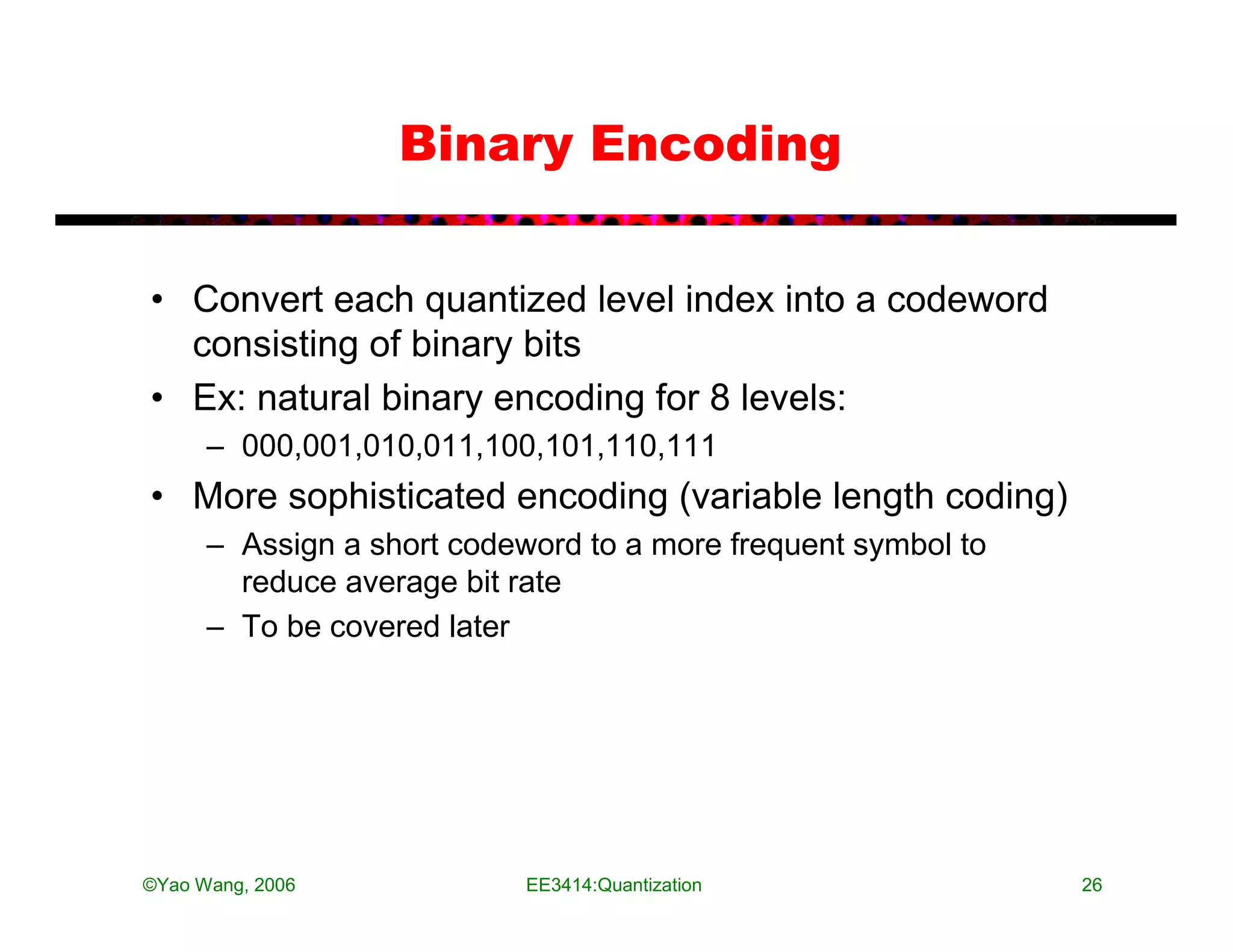
• Binary Encoding
– Convert each quantized value into a binary codeword
©Yao Wang, 2006 EE3414:Quantization 3](https://image.slidesharecdn.com/13642991-120715025628-phpapp02/75/quantization-3-2048.jpg)
![µ-Law Quantization
y =F [ x ]
|x|
log 1+µ
X max
.sign[ x]
= X max
log[1 + µ ]
©Yao Wang, 2006 EE3414:Quantization 17](https://image.slidesharecdn.com/13642991-120715025628-phpapp02/75/quantization-17-2048.jpg)
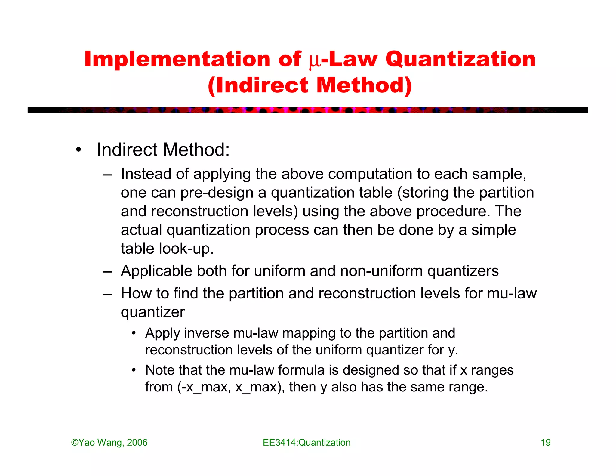
![Implementation of µ-Law Quantization
(Direct Method)
– Transform the signal using µ-law: x->y
y =F [ x ]
|x|
log 1+µ
X max
= X max .sign[ x]
log[1 + µ ]
– Quantize the transformed value using a uniform quantizer: y->y^
– Transform the quantized value back using inverse µ-law: y^->x^
x =F −1[ y ]
X log(1+ µ ) y
= max 10 X max − 1 sign(y)
µ
©Yao Wang, 2006 EE3414:Quantization 18](https://image.slidesharecdn.com/13642991-120715025628-phpapp02/75/quantization-18-2048.jpg)
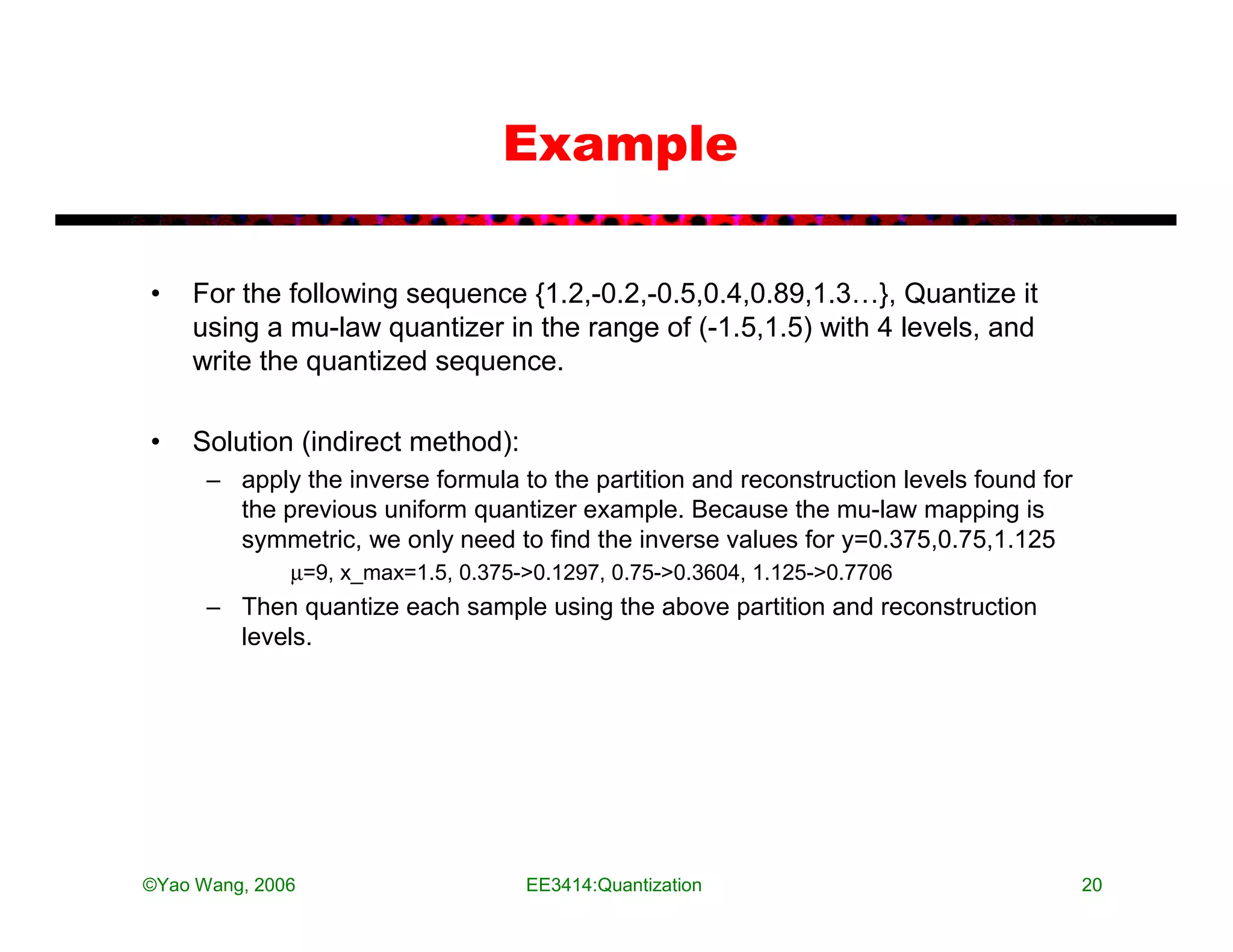
![Example (cntd)
-1.125 -0.375 0.375 1.125
-1.5 -0.75 0 0.75 1.5
x =F −1[ y ]
Inverse µ-law
X log(1+ µ ) y
= max 10 X max − 1 sign(y)
µ
-0.77 -0.13 0.13 0.77
-1.5 -0.36 0 0.36 1.5
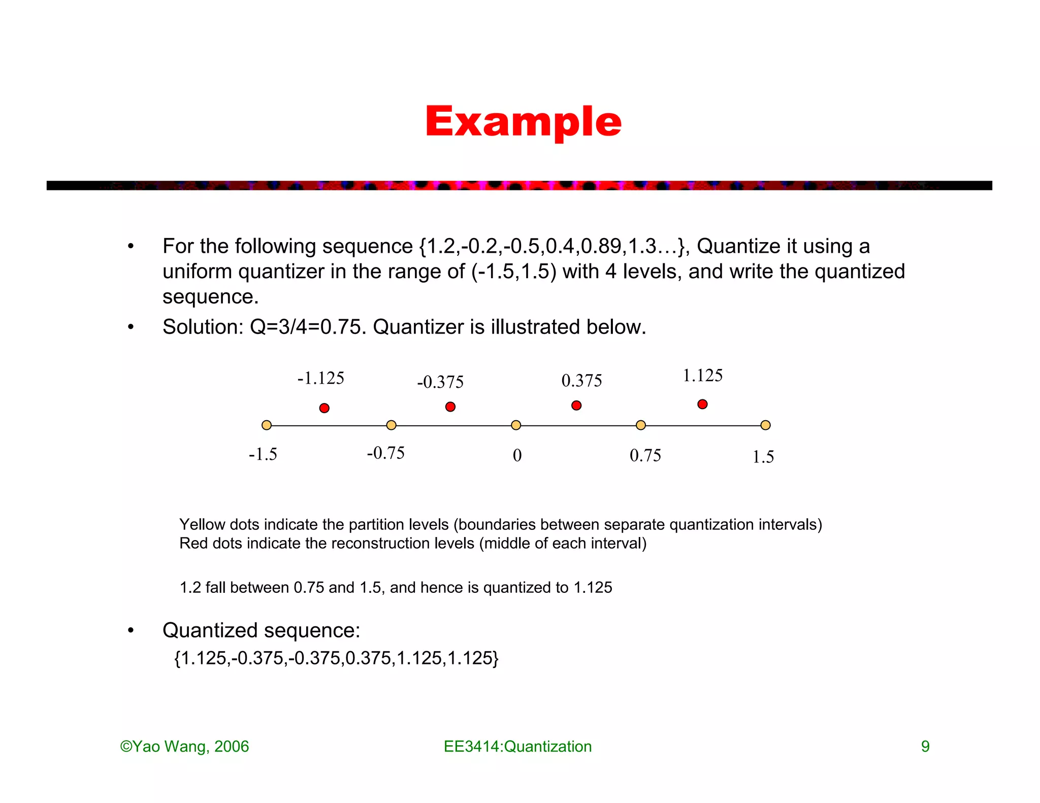
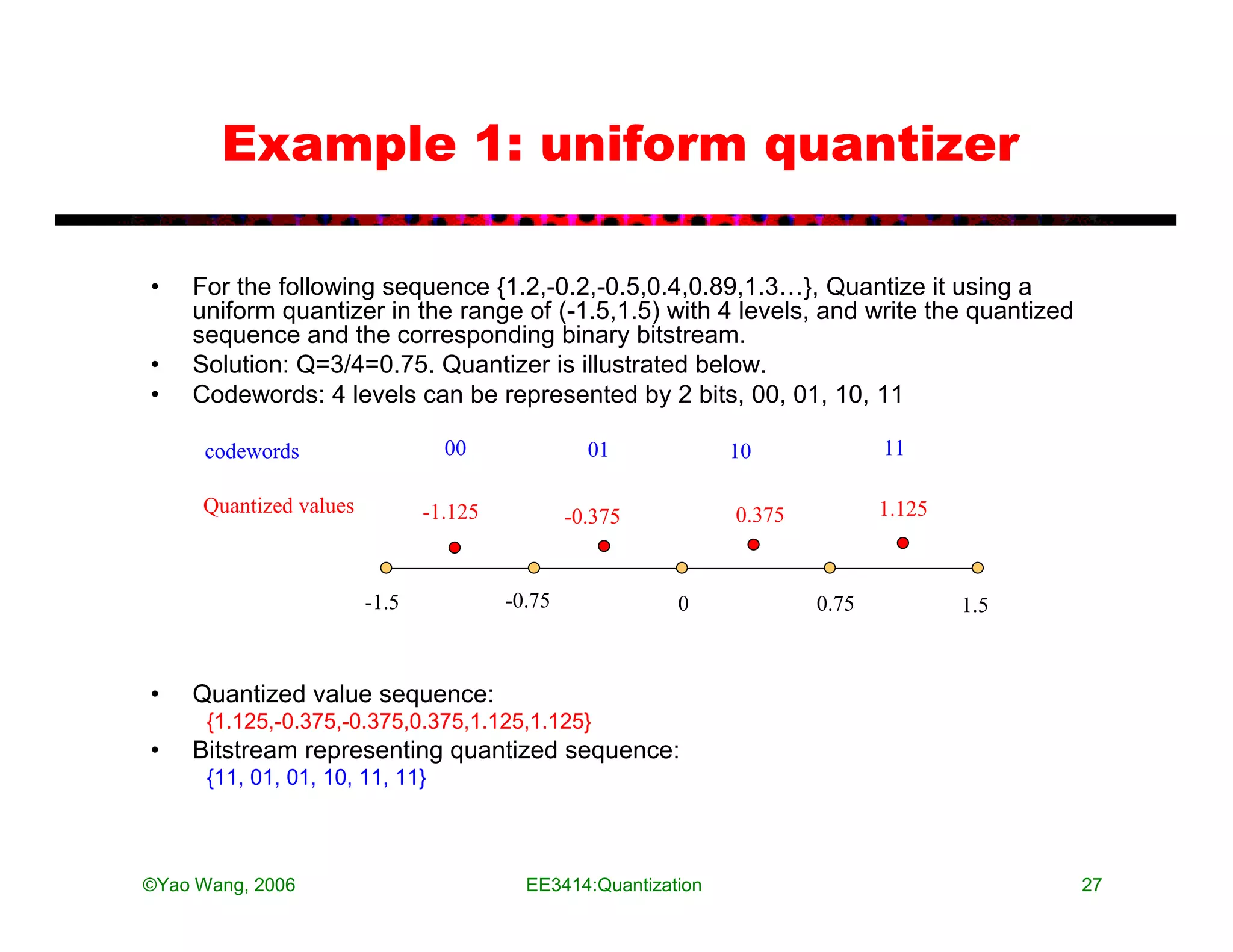
• Original sequence: {1.2,-0.2,-0.5,0.4,0.89,1.3…}
• Quantized sequence
– {0.77,-0.13,-0.77,0.77,0.77,0.77}
©Yao Wang, 2006 EE3414:Quantization 21](https://image.slidesharecdn.com/13642991-120715025628-phpapp02/75/quantization-21-2048.jpg)
![Example 2: mu-law quantizer
codewords 00 01 10 11
-1.125 -0.375 0.375 1.125
-1.5 -0.75 0 0.75 1.5
x =F −1[ y ]
Inverse µ-law
X log(1+ µ ) y
= max 10 X max − 1 sign(y)
codewords 00 01 10 11 µ
-0.77 -0.13 0.13 0.77
-1.5 -0.36 0 0.36 1.5
• Original sequence: {1.2,-0.2,-0.5,0.4,0.89,1.3…}
• Quantized sequence: {0.77,-0.13,-0.77,0.77,0.77,0.77}
• Bitstream: {11,01,00,11,11,11}
©Yao Wang, 2006 EE3414:Quantization 28](https://image.slidesharecdn.com/13642991-120715025628-phpapp02/75/quantization-28-2048.jpg)
![Bit Rate of a Digital Sequence
• Sampling rate: f_s sample/sec
• Quantization resolution: B bit/sample, B=[log2(L)]
• Bit rate: R=f_s B bit/sec
• Ex: speech signal sampled at 8 KHz, quantized to 8 bit/sample,
R=8*8 = 64 Kbps
• Ex: music signal sampled at 44 KHz, quantized to 16 bit/sample,
R=44*16=704 Kbps
• Ex: stereo music with each channel at 704 Kbps: R=2*704=1.4
Mbps
• Required bandwidth for transmitting a digital signal depends on
the modulation technique.
– To be covered later.
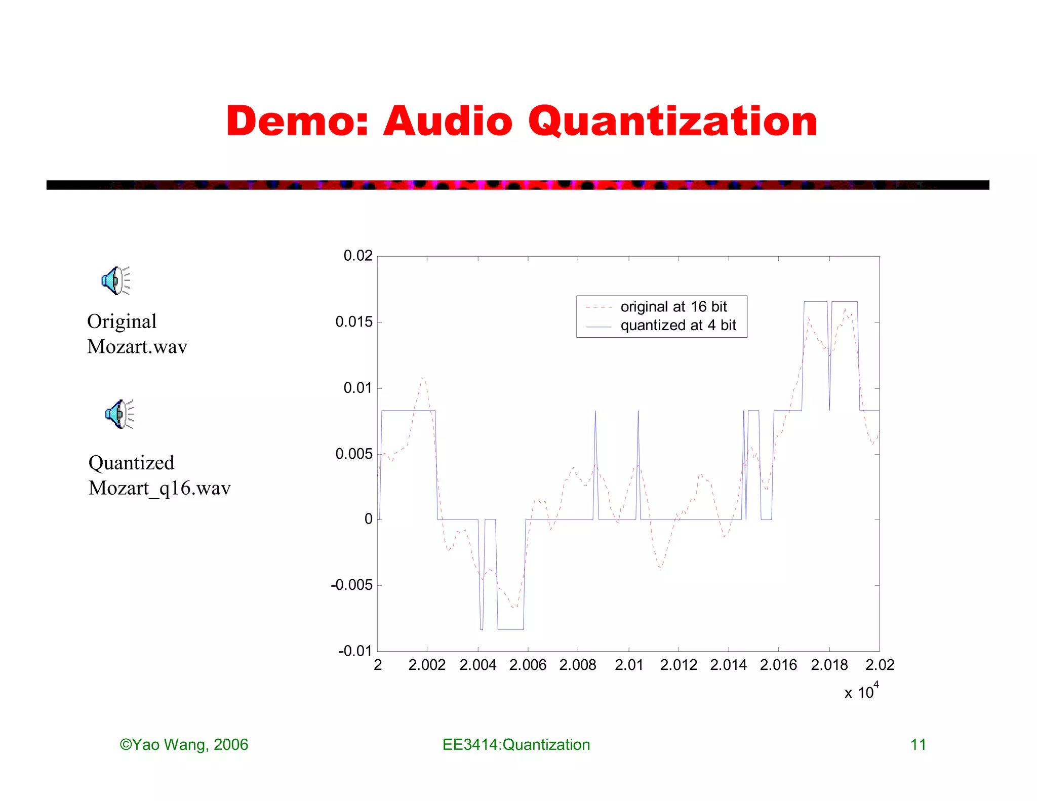
• Data rate of a multimedia signal can be reduced significantly
through lossy compression w/o affecting the perceptual quality.
– To be covered later.
©Yao Wang, 2006 EE3414:Quantization 29](https://image.slidesharecdn.com/13642991-120715025628-phpapp02/75/quantization-29-2048.jpg)

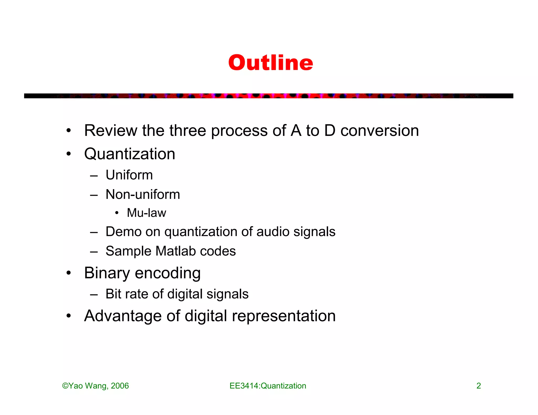
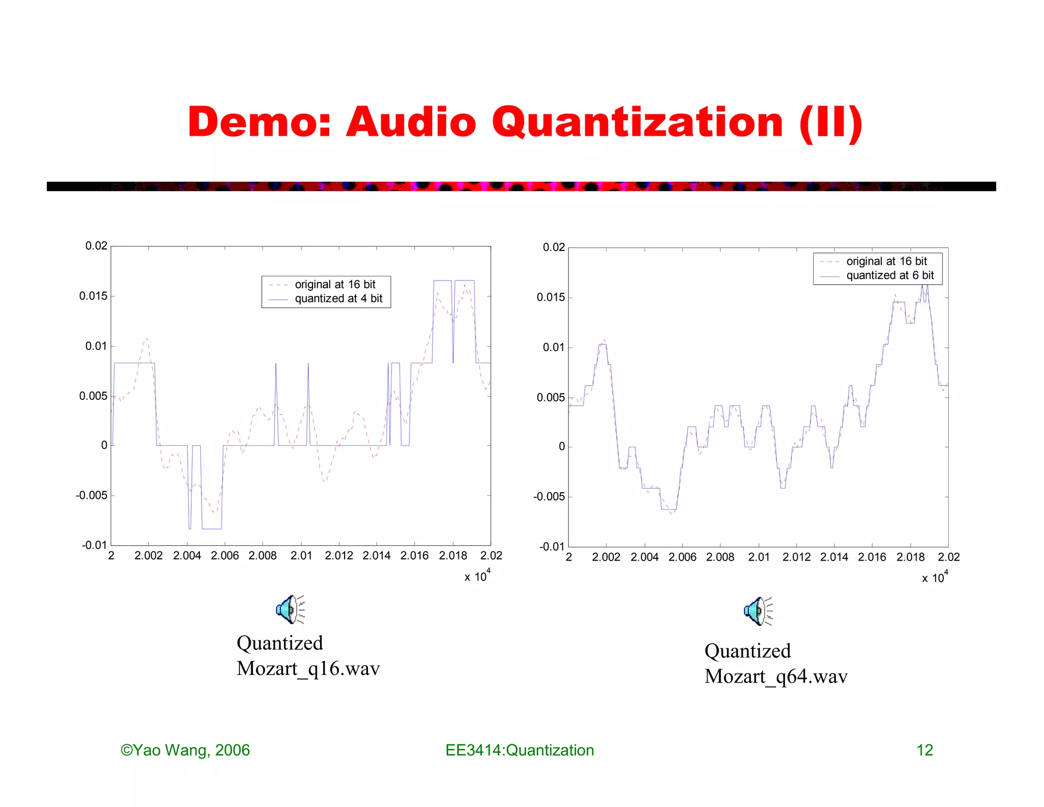
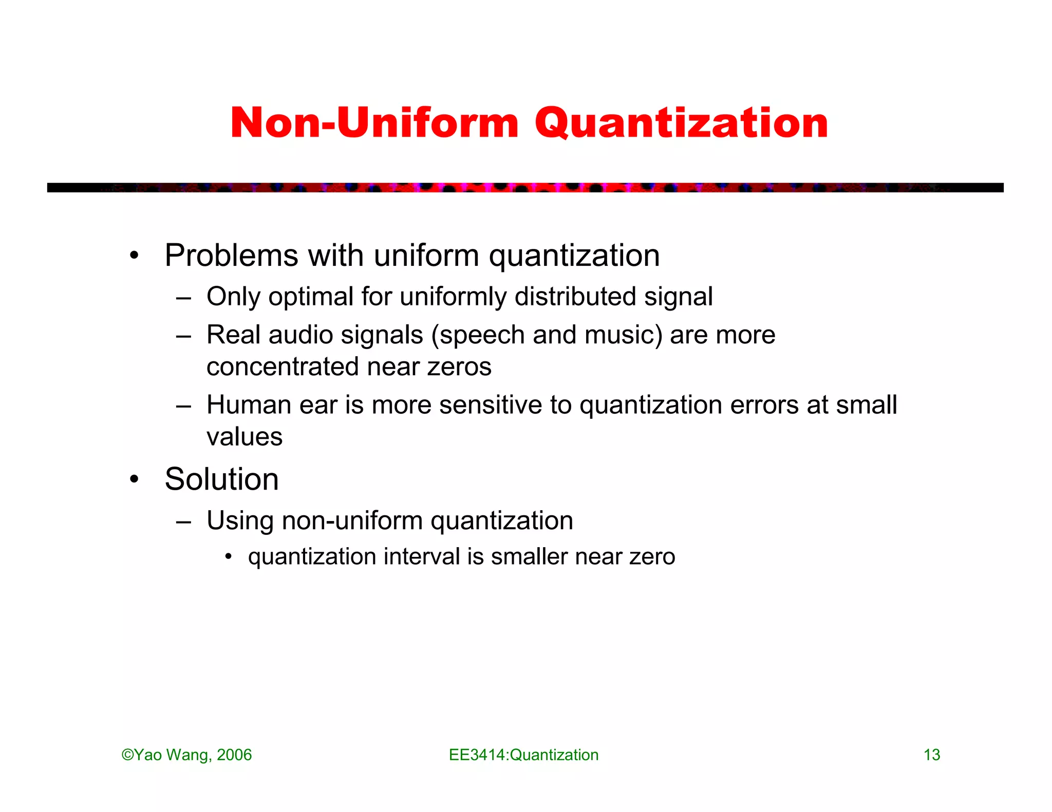
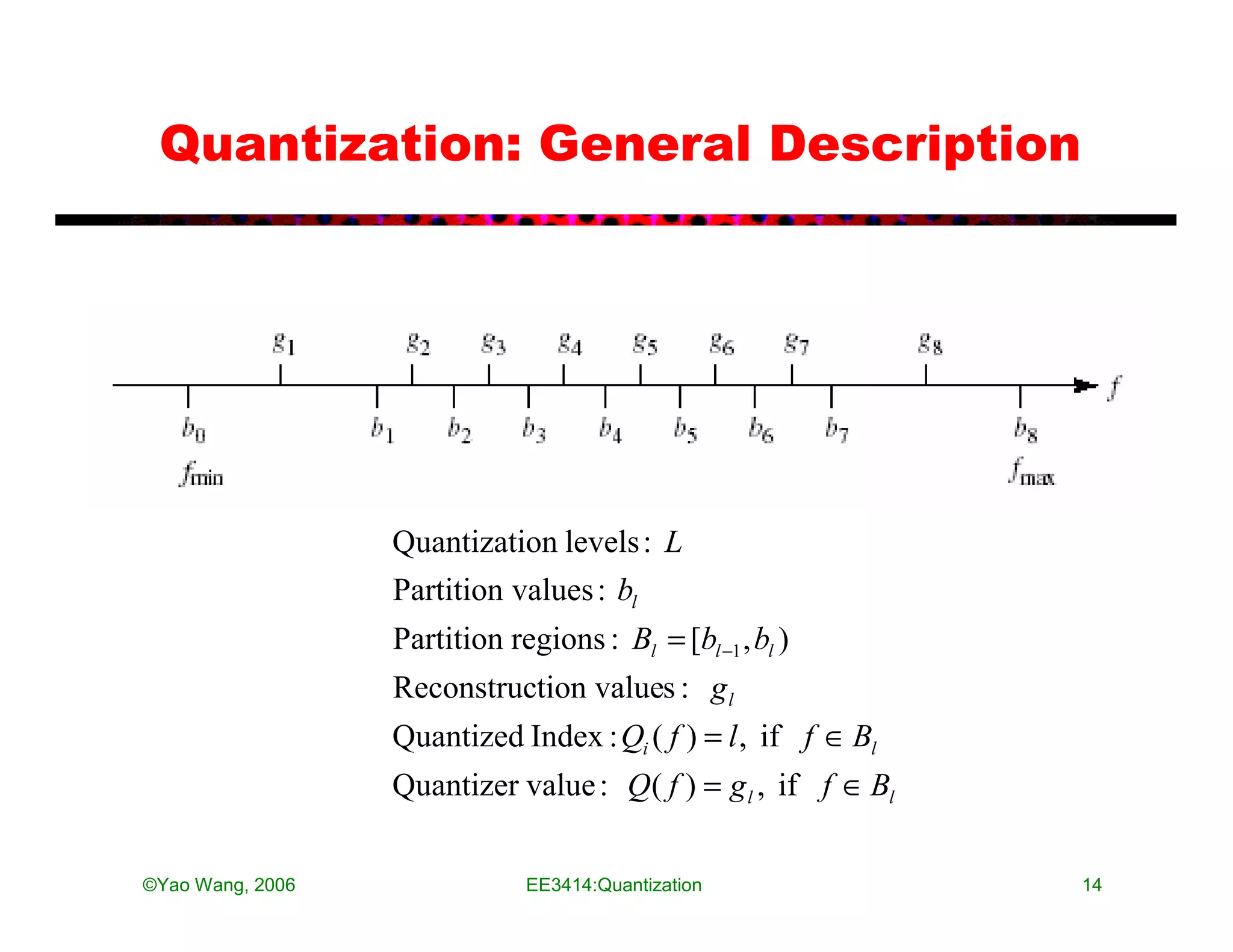
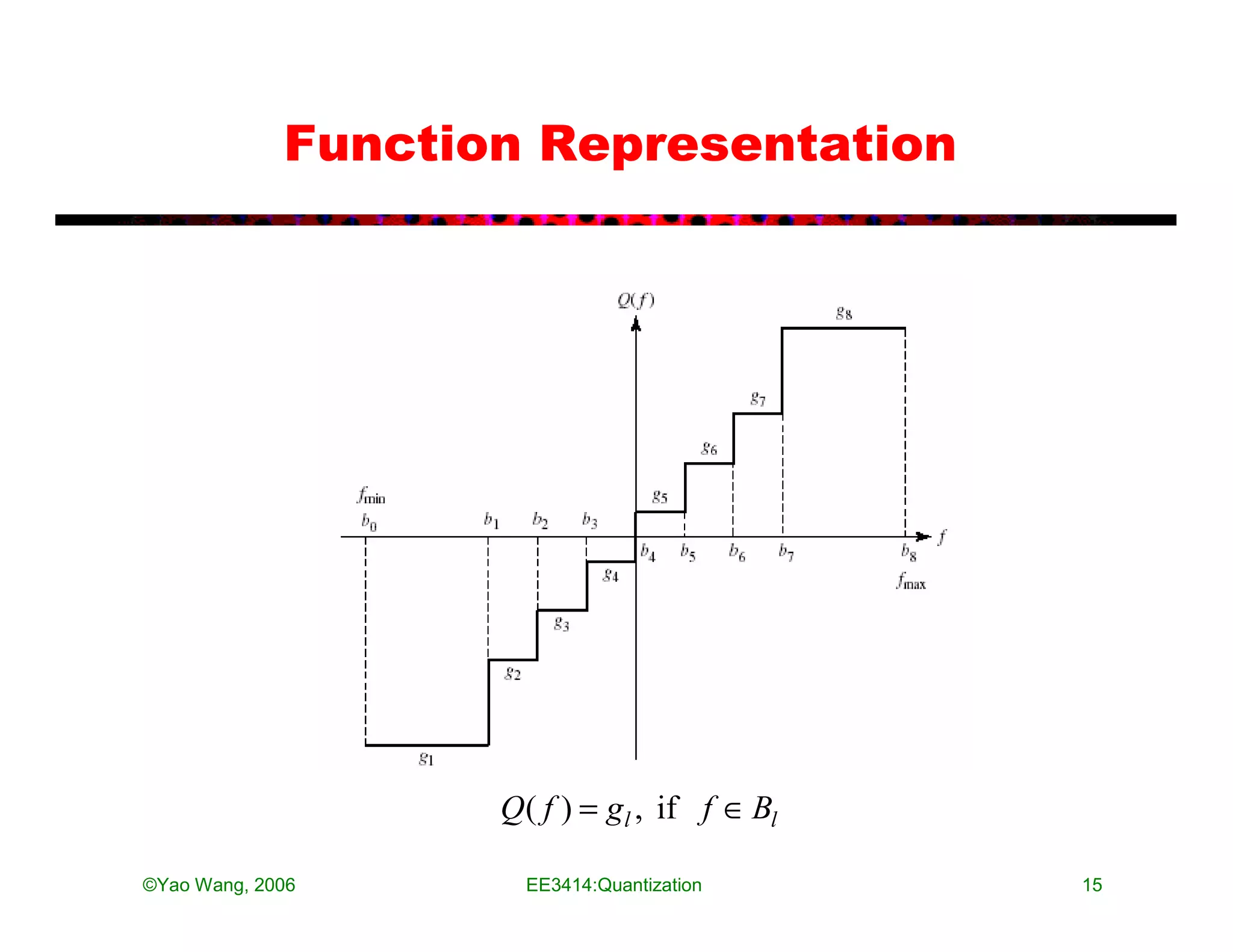
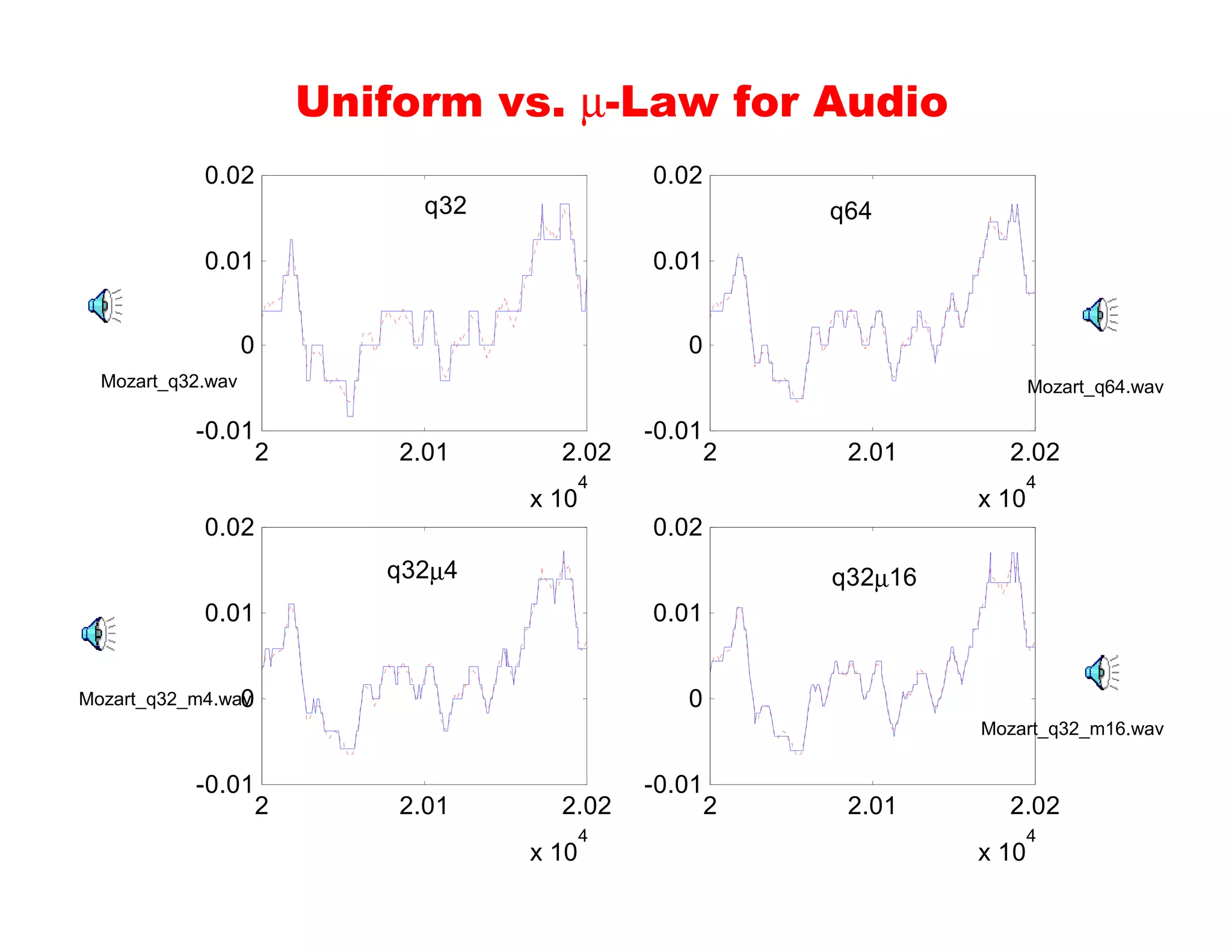
The document discusses quantization in analog-to-digital conversion. It describes the three processes of A/D conversion as sampling, quantization, and binary encoding. Quantization involves mapping amplitude values into a set of discrete values using a quantization interval or step size. The document discusses uniform quantization and how the range is divided into equal intervals. It also discusses non-uniform quantization which has smaller intervals near zero to better match real audio signals. Examples and MATLAB code demonstrations are provided to illustrate quantization of audio signals at different bit rates.


![Digital Signal Processing[ECEG-3171]-Ch1_L02](https://cdn.slidesharecdn.com/ss_thumbnails/dspl2-180427094423-thumbnail.jpg?width=640&height=640&fit=bounds)