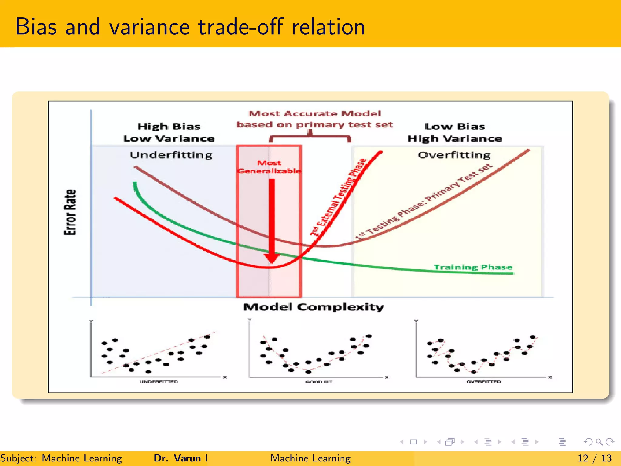
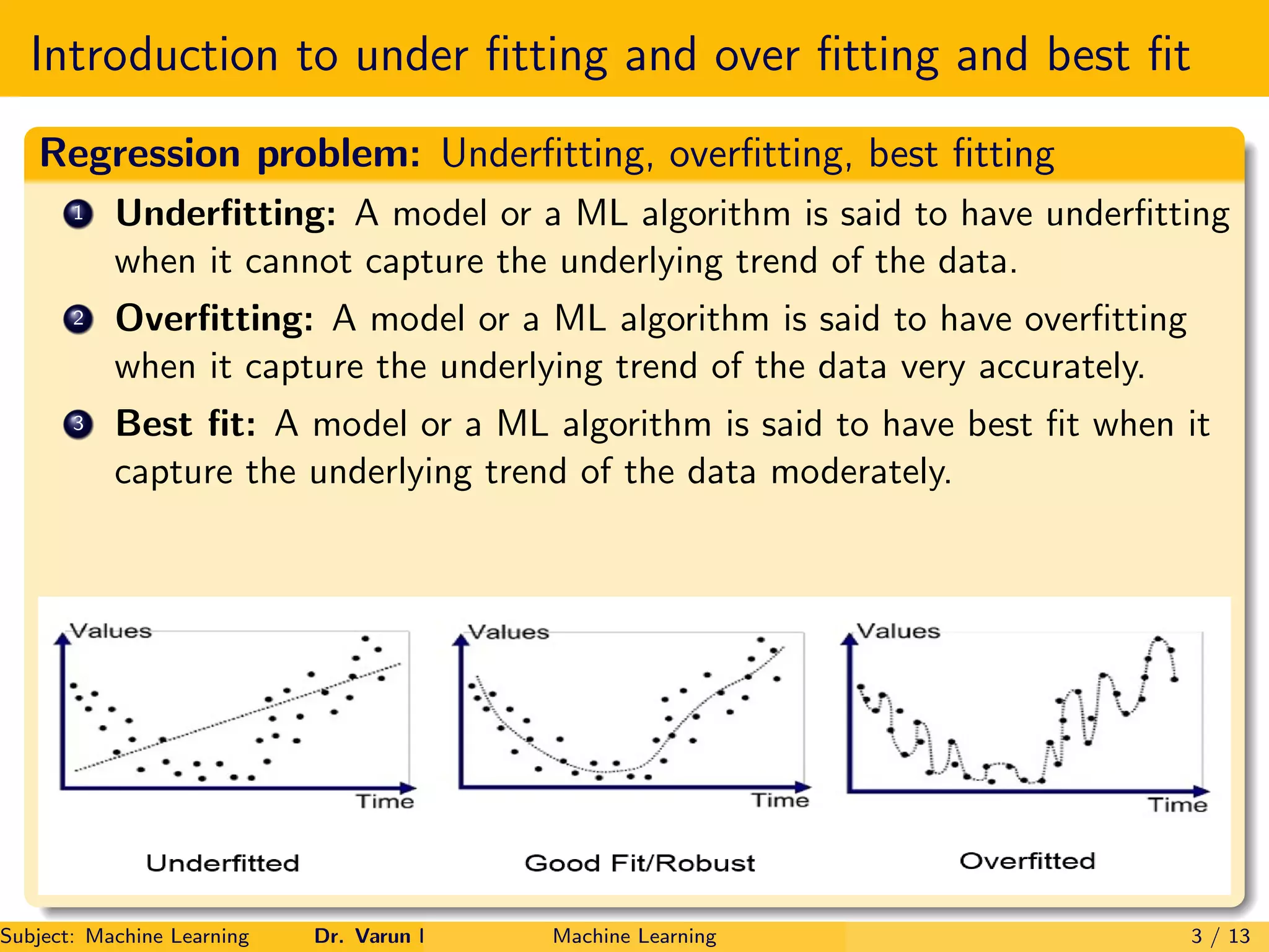
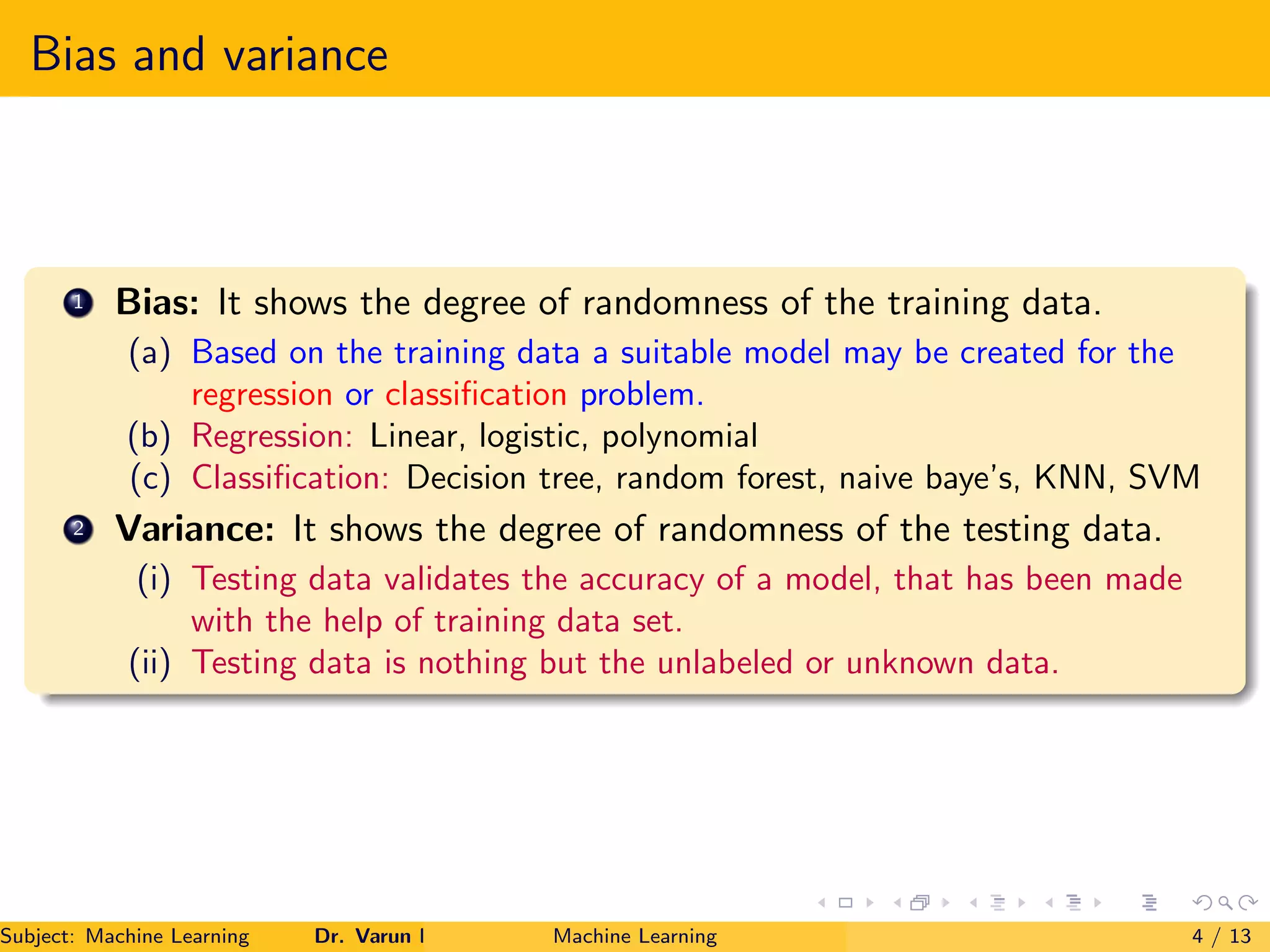
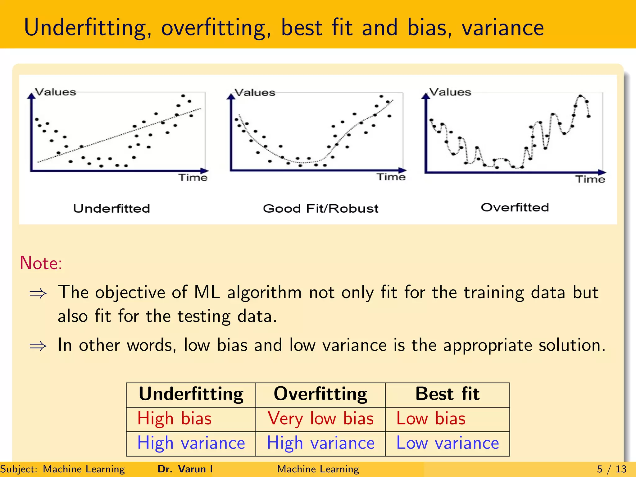
The document explores the bias-variance trade-off in machine learning, focusing on underfitting, overfitting, and best fit models. It defines bias as the error due to the complexity of the model in relation to training data, while variance refers to the error due to the model's performance on testing data. The goal is to achieve a model with low bias and low variance for optimal performance.

1. Bias Variance Trade-off in Machine Learning
Subject: Machine Learning
Dr. Varun Kumar
Subject: Machine Learning Dr. Varun Kumar Machine Learning 1 / 13

2. Outlines
1 Introduction to Under Fitting and Over Fitting
2 Introduction to Bias and Variance
3 Mathematical Intuition
4 Bias Variance Trade-off relation
5 References
Subject: Machine Learning Dr. Varun Kumar Machine Learning 2 / 13

3. Introduction to under fitting and over fitting and best fit
Regression problem: Underfitting, overfitting, best fitting
1 Underfitting: A model or a ML algorithm is said to have underfitting
when it cannot capture the underlying trend of the data.
2 Overfitting: A model or a ML algorithm is said to have overfitting
when it capture the underlying trend of the data very accurately.
3 Best fit: A model or a ML algorithm is said to have best fit when it
capture the underlying trend of the data moderately.
Subject: Machine Learning Dr. Varun Kumar Machine Learning 3 / 13

4. Bias and variance
1 Bias: It shows the degree of randomness of the training data.
(a) Based on the training data a suitable model may be created for the
regression or classification problem.
(b) Regression: Linear, logistic, polynomial
(c) Classification: Decision tree, random forest, naive baye’s, KNN, SVM
2 Variance: It shows the degree of randomness of the testing data.
(i) Testing data validates the accuracy of a model, that has been made
with the help of training data set.
(ii) Testing data is nothing but the unlabeled or unknown data.
Subject: Machine Learning Dr. Varun Kumar Machine Learning 4 / 13

5. Underfitting, overfitting, best fit and bias, variance
Note:
⇒ The objective of ML algorithm not only fit for the training data but
also fit for the testing data.
⇒ In other words, low bias and low variance is the appropriate solution.
Underfitting Overfitting Best fit
High bias Very low bias Low bias
High variance High variance Low variance
Subject: Machine Learning Dr. Varun Kumar Machine Learning 5 / 13

6. Underfitting, overfitting, and best fit in classification problem
A classifier (Decision tree, random forest, naive baye’s, KNN, SVM) works
on two types of data
Training data
Testing data
Example:
Classifier comes under the category of underfitting, overfitting, and best fit
based on its training and testing accuracy.
Underfitting Overfitting Best fit
Train error=25% Train error=1% Train error=8%
Test error= 27% Test error= 23% Test error=9%
Subject: Machine Learning Dr. Varun Kumar Machine Learning 6 / 13

7. Mathematical intuition
bias ˆ
f (x)
= E[ˆ
f (x)] − f (x) (1)
variance ˆ
f (x)
= E
h
ˆ
f (x) − E[ˆ
f (x)]
2
i
(2)
⇒ ˆ
f (x) → output observed through the training model
⇒ For linear model ˆ
f (x) = w1x + w0
⇒ For complex model ˆ
f (x) =
Pp
i=1 wi xi + w0
⇒ We don’t have idea regarding the true f (x).
⇒ Simple model: Low bias high variance
⇒ Complex model: High bias low variance
E[(y − ˆ
f (x))2
] = bias2
+ Variance + σ2
(Irreducible error) (3)
Subject: Machine Learning Dr. Varun Kumar Machine Learning 7 / 13

8. Continued–
⇒ Let there be n + m sample data in a given data set in which n and m
samples are taken for the training and testing (validation) purpose then
trainerr =
1
n
n
X
i=1
(yi − ˆ
f (xi ))2
testerr =
1
m
n+m
X
i=n+1
(yi − ˆ
f (xi ))2
⇒ If model complexity is increased the training model becomes too optimistic
gives a wrong picture of how close ˆ
f to f .
⇒ Let D = {xi , yi }n+m
1 is a given data set, where
yi = f (xi ) + i
⇒ ∼ N(0, σ2
)
Subject: Machine Learning Dr. Varun Kumar Machine Learning 8 / 13

9. Continued–
⇒ We use ˆ
f to approximate f , where training set T ⊂ D such that
yi = ˆ
f (xi )
⇒ We are interested to know
E
h
ˆ
f (xi ) − f (xi )
2
i
⇒ We cannot estimate the above expression directly, because we don’t know
f (xi )
E
(ŷi − yi )2
= E
(ˆ
f (xi ) − f (xi ) − i )2
⇐ yi = f (xi ) + i
= E
(ˆ
f (xi ) − f (xi ))2
− 2i (ˆ
f (xi ) − f (xi )) + 2
i
= E
(ˆ
f (xi ) − f (xi ))2
− 2E
i (ˆ
f (xi ) − f (xi ))
+ E
2
i
E
(ˆ
f (xi ) − f (xi ))2
= E
(ŷi − yi )2
+ 2E
i (ˆ
f (xi ) − f (xi ))
− E
2
i
(4)
Subject: Machine Learning Dr. Varun Kumar Machine Learning 9 / 13

10. Continued–
⇒ Empirical estimate: Let Z = {zi }n
i=1
E(Z) =
1
n
n
X
i=1
zi
⇒ We can empirically evaluate R.H.S using training or test observation
Case 1: Using test observation:
E
(ˆ
f (xi ) − f (xi ))2
| {z }
True error
= E
(ŷi − yi )2
+ 2E
i (ˆ
f (xi ) − f (xi ))
− E
2
i
=
1
m
n+m
X
i=n+1
(ŷi − yi )2
| {z }
Empirical error
−
1
m
n+m
X
i=n+1
(i )2
| {z }
Small constant
+ 2E
h
i (ˆ
f (xi ) − f (xi ))
i
| {z }
Covariance
∵ Cov(X, Y ) = E
h
(X − µx )(Y − µy )
i
let i = X and Y = (ˆ
f (xi ) − f (xi ))
Subject: Machine Learning Dr. Varun Kumar Machine Learning 10 / 13

11. Continued–
⇒ E
h
(X − µx )(Y − µy )
i
= E
h
X(Y − µy )
i
= E
XY
− µy E
X
= E[XY ]
⇒ None of the test data participated for estimating the ˆ
f (xi ).
⇒ ˆ
f (xi ) is estimated only using the training data.
⇒ ∴ i ⊥ (ˆ
f (xi ) − f (xi ))
∴ E[XY ] = E[X]E[Y ] = 0
⇒ True error=Empirical error+Small constant ← Test data
Case 2: For training observation:
E[XY ] 6= 0
Using Stein’s Lemma
1
n
n
X
i=1
i (ˆ
f (xi ) − f (xi )) =
σ2
n
n
X
i=1
∂ ˆ
f (xi )
∂yi
Subject: Machine Learning Dr. Varun Kumar Machine Learning 11 / 13

12. Bias and variance trade-off relation
Subject: Machine Learning Dr. Varun Kumar Machine Learning 12 / 13

13. References
E. Alpaydin, Introduction to machine learning. MIT press, 2020.
J. Grus, Data science from scratch: first principles with python. O’Reilly Media,
2019.
T. M. Mitchell, The discipline of machine learning. Carnegie Mellon University,
School of Computer Science, Machine Learning , 2006, vol. 9.
Subject: Machine Learning Dr. Varun Kumar Machine Learning 13 / 13