Downloaded 147 times


![Bias Variance Decomposition
• Training set of points: 𝑥(1), 𝑥(2). . 𝑥(𝑚)
• Assume function 𝑦 = 𝑓 𝑥 + 𝜀 with noise 𝜀 with 0 mean and variance 𝜎2
• Goal: Find function 𝑓(𝑥) that approximates the true function 𝑓 𝑥 so as to
minimize (𝑦 − 𝑓 𝑥 ) 2
• Note: 𝑉𝑎𝑟 𝑋 = 𝐸 𝑋2 − 𝐸[𝑋]2
• Note: 𝐸[𝜀]=0, 𝐸[𝑦]=𝐸[𝑓 + 𝜀]=𝐸 𝑓 = f
• Note: 𝑉𝑎𝑟 𝑦 = 𝐸 𝑦 − 𝐸 𝑦 2 = 𝐸 𝑦 − 𝑓 2 = 𝐸 𝑓 + 𝜀 − 𝑓 2 =𝜎2](https://image.slidesharecdn.com/hyperparametertuningweek3-units4-5-181123231509/85/Hyperparameter-Tuning-15-320.jpg)
![Bias Variance Decomposition
𝐸 𝑦 − 𝑓
2
= 𝐸 𝑦2 + 𝑓2 − 2𝑦 𝑓
= 𝐸 𝑦2
+ 𝐸 𝑓2
− 2𝐸[𝑦 𝑓]
= 𝑉𝑎𝑟 𝑦 + 𝐸[𝑦]2 + 𝑉𝑎𝑟 𝑓 + 𝐸[ 𝑓]2 − 2𝑓𝐸[ 𝑓]
= 𝑉𝑎𝑟 𝑦 + 𝑉𝑎𝑟[ 𝑓]+(𝑓2
− 2𝑓𝐸[ 𝑓]+𝐸[ 𝑓2
])
= 𝑉𝑎𝑟 𝑦 + 𝑉𝑎𝑟 𝑓 +(𝑓 − 𝐸[ 𝑓]) 2
𝐸 𝑦 − 𝑓
2
= 𝜎2 + 𝑉𝑎𝑟 𝑓 + 𝐵𝑖𝑎𝑠[ 𝑓]
2
Average test error over large ensemble of training sets](https://image.slidesharecdn.com/hyperparametertuningweek3-units4-5-181123231509/85/Hyperparameter-Tuning-16-320.jpg)


 and perform the
following steps:
• Feedforward: For each l=1, 2, 3, … L compute 𝒛[𝑙](𝑥) = 𝒘[𝑙] 𝒂 𝑙−1 (𝑥) + 𝒃[𝑙] and 𝒂[𝑙](𝑥) =
𝜎(𝒛 𝑙
)
• Output Error: Compute 𝜺[𝐿](𝑥) = 𝜵 𝒂 𝐽⨀𝜎′(𝒛[𝐿](𝑥))
• Backpropagate Error: For each i=L-l, L-2 , … 1 compute 𝜺[𝑙](𝑥) =
((𝒘[𝑙+1]) 𝑇 𝜺[𝑙+1](𝑥))⨀𝜎′(𝒛[𝑙](𝑥))
• Compute One Step Of Gradient Descent: For each l=L, L-1, L-2, … 1, update the
weights according to the rules:
• 𝒘𝑙
= 𝒘𝑙
−
∝
𝑚 𝑥 𝜺 𝑙 𝑥
(𝒂 𝑙−1 𝑥
) 𝑇
• 𝒃𝑙
= 𝒃𝑙
−
𝛼
𝑚 𝑥 𝜺 𝑙 𝑥
Controls how fast learning occurs for 𝒘𝑙
Controls how fast learning occurs for 𝒃𝑙](https://image.slidesharecdn.com/hyperparametertuningweek3-units4-5-181123231509/85/Hyperparameter-Tuning-39-320.jpg)


![Mini-Batch Gradient Descent
• Solution:
• Divide training set into smaller mini-batches:
• 𝑿 = [𝑋1
, 𝑋2
, 𝑋3
, . . . 𝑋 𝑏
| 𝑋 𝑏+1
, 𝑋 𝑏+2
, 𝑋 𝑏+3
, . . . 𝑋2𝑏
|. . . 𝑋 𝑚−1 𝑏+1
… 𝑋 𝑚
• 𝒀 = [𝑌1
, 𝑌2
, 𝑌3
, . . . 𝑌 𝑏
| 𝑌 𝑏+1
, 𝑌 𝑏+2
, 𝑌 𝑏+3
, . . . 𝑌2𝑏
|. . . |𝑌 𝑚−1 𝑏+1
… 𝑌 𝑚
]
• Each 𝑿{𝑖}
has dimension (nx, b)
• Each 𝒀{𝑖}
has dimension (1, b)
𝑿{1}
𝑿{2} 𝑿{𝑚/𝑏}
𝒀{1}
𝒀{1} 𝒀{𝑚/𝑏}](https://image.slidesharecdn.com/hyperparametertuningweek3-units4-5-181123231509/85/Hyperparameter-Tuning-45-320.jpg)

![Mini-Batch Gradient Descent
Pseudo-Code
For j=1. . .E (number of epochs)
For t=1 …b{
Forward prop on 𝑿{𝑡}
𝒁[1]
= 𝑾[1]
𝑿{𝑡}
+ 𝒃[1]
𝑨[1]
= 𝒈 1
𝒁 1
…
𝑨[𝐿]
= 𝒈 𝐿
𝒁 𝐿
𝐽{𝑡}
=
1
𝑏 𝑖=1
𝑏
𝐿( 𝒚 𝑖
, 𝒚 𝑖
)+
𝜆
2∗𝑏 𝑙 ||𝒘𝑙
2
|| 𝐹
Backpropagation to compute gradients with respect to 𝐽{𝑡}
𝒘𝑙
= 𝒘𝑙
-𝛼𝑑𝒘𝑙
𝒃𝑙
= 𝒃𝑙
-𝛼𝑑𝒃𝑙
}
}
1 epoch](https://image.slidesharecdn.com/hyperparametertuningweek3-units4-5-181123231509/85/Hyperparameter-Tuning-47-320.jpg)


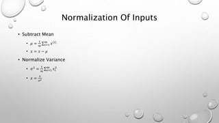
![Batch Motivation Concept
What if we could normalize the activations: 𝒂[𝑙] so that the training of 𝑾[𝑙+1] and 𝒃[𝑙+1] is more e
That is, can we normalize the activations in the hidden layers too such that training of paramet
layers may happen more rapidly?
In practice, 𝒛𝑙 is normalized.](https://image.slidesharecdn.com/hyperparametertuningweek3-units4-5-181123231509/85/Hyperparameter-Tuning-73-320.jpg)

, 𝒛[𝑙](2)
. . . 𝒛[𝑙](𝑚)
Subtract Mean
𝒛(𝑖)
=
1
𝑚
𝑖=1
𝑚
𝒛(𝑖)
Normalize Variance
𝒖 =
1
𝑚
𝑖
𝒛(𝑖)
𝜎2 =
1
𝑚
𝑖=1
𝑚
(𝒛 𝑖 − 𝝁 𝑖 )2
𝒛 𝑛𝑜𝑟𝑚
(𝑖)
=
𝒛(𝑖)
− 𝝁
𝜎2 + 𝜖
𝒛(𝑖)
= 𝛾 𝒛 𝑛𝑜𝑟𝑚
(𝑖)
+𝛽
This will have mean 0 and variance 1.
But, we don’t always want that. For
example, we may want to cluster
values near non-linear region of
activation function to take advantage
of non-linearity.
𝛾 and 𝛽 are learnable parameters learned
via gradient descent for example.
If 𝛾 = 𝜎2 + 𝜖
and 𝛽 = 𝜇:
𝒛(𝑖)
= 𝒛(𝑖)
𝛾 and 𝛽 control mean and varian](https://image.slidesharecdn.com/hyperparametertuningweek3-units4-5-181123231509/85/Hyperparameter-Tuning-74-320.jpg)

![Notes on Batch Normalization
• Batch normalization is done over mini-batches
• 𝒛[𝑙] = 𝑾[𝑙−1] 𝒛[𝑙] + 𝑏[𝑙]
• 𝛽[𝑙]
𝑎𝑛𝑑 𝛾[𝑙]
have dimensions (𝑛[𝑙]
, 1)
Will be set to 0 in mean subtraction step so we can eliminate b
as parameter. Beta effectively replaces b.](https://image.slidesharecdn.com/hyperparametertuningweek3-units4-5-181123231509/85/Hyperparameter-Tuning-76-320.jpg)
![Batch Normalization PseudoCode
• For t=1…Number of Mini-Batches
• Compute forward prop on each 𝑋{𝑡}
• In each hidden layer use batch normalization to compute 𝒛[𝑙]
from 𝒛[𝑙]
• Use backpropagation to compute 𝑑𝑾[𝑙]
, 𝑑𝛽[𝑙]
, 𝑑𝛾[𝑙]
• Update parameters:
• 𝑾[𝑙]
= 𝑾[𝑙]
− 𝛼𝑑𝑾[𝑙]
• 𝛽[𝑙]
= 𝛽[𝑙]
− 𝛼𝑑𝛽[𝑙]
• 𝛾[𝑙]
= 𝛾[𝑙]
− 𝛼𝑑𝛾[𝑙]
This will work with momentum, RMSProp and Adam for example.](https://image.slidesharecdn.com/hyperparametertuningweek3-units4-5-181123231509/85/Hyperparameter-Tuning-77-320.jpg)


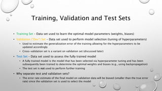
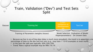
The document discusses hyperparameters and hyperparameter tuning in deep learning models. It defines hyperparameters as parameters that govern how the model parameters (weights and biases) are determined during training, in contrast to model parameters which are learned from the training data. Important hyperparameters include the learning rate, number of layers and units, and activation functions. The goal of training is for the model to perform optimally on unseen test data. Model selection, such as through cross-validation, is used to select the optimal hyperparameters. Training, validation, and test sets are also discussed, with the validation set used for model selection and the test set providing an unbiased evaluation of the fully trained model.