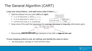
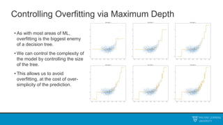
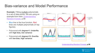
The document discusses decision trees and ensemble methods. It begins with an agenda that covers the bias-variance tradeoff, generalizations of this concept, the ExtraTrees algorithm, its sklearn interface, and conclusions. It then reviews decision trees, plotting sample data and walking through how the tree would split the data. Next, it covers the general CART algorithm and different impurity measures. It discusses controlling overfitting via tree depth and other techniques. Finally, it delves into explaining the bias-variance decomposition and tradeoff in more detail.


![The Setup I
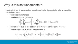
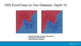
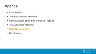
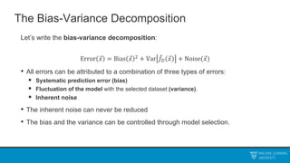
• Suppose I have a regression problem where I take in vectors 𝑥𝑖 and try to make
predictions of a single value 𝑦𝑖. Suppose for the moment that we know the
absolute true answer up to an independent random noise:
𝑦 = 𝑓 𝑥 + 𝜖(𝑥)
• The noise should be independent from any randomness inherent in 𝑥, and should
have mean zero, so that 𝑓 is the best possible guess.
• The function 𝑓 is deterministic. You can think of it as averaging the answer over
the true distribution in the world for that input:
𝑓 𝑥 = 𝔼[𝑦|𝑥]](https://image.slidesharecdn.com/mludtelecture2-230212190438-a3f17b7c/85/MLU_DTE_Lecture_2-pptx-21-320.jpg)
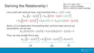
![Deriving the Relationship II
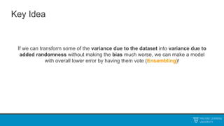
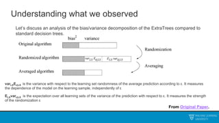
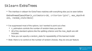
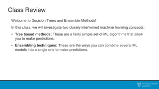
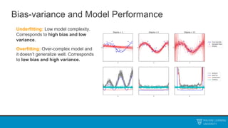
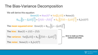
Now, let 𝑓(𝑥) = 𝔼𝒟[𝑓𝒟 𝑥 ] denote the average prediction of the ML model over every
training set. We may write:
𝔼𝒟 𝑓 𝑥 − 𝑓𝒟 𝑥
2
= 𝔼𝒟 𝑓 𝑥 − 𝑓 𝑥 + 𝑓 𝑥 − 𝑓𝒟 𝑥
2
= 𝔼𝒟 𝑓 𝑥 − 𝑓 𝑥
2
+ 𝔼𝒟 𝑓 𝑥 − 𝑓𝒟 𝑥
2
+2 ⋅ 𝔼𝑦,𝒟 𝑓 𝑥 − 𝑓 𝑥 𝑓 𝑥 − 𝑓𝒟 𝑥
Thus the last term is zero.
Also note 𝑓 𝑥 − 𝑓 𝑥 is not random, so the expectation does nothing on the left.
Doesn’t depend on
the dataset
Mean zero when
averaged over 𝒟
(2)
E 𝑋 + 𝑌 = 𝐸 𝑋 + 𝐸 𝑌
E 𝑎 𝑋 = 𝑎 𝐸 𝑋 , a: Constant
E 𝑋 𝑌 = 𝐸 𝑋 𝐸 𝑌 , X and Y are indep.](https://image.slidesharecdn.com/mludtelecture2-230212190438-a3f17b7c/85/MLU_DTE_Lecture_2-pptx-24-320.jpg)
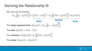
![Deriving the Relationship II
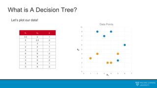
Now, let 𝑓(𝑥) = 𝔼𝒟[𝑓𝒟 𝑥 ] denote the average prediction of the ML model over every
training set. We may write:
𝔼𝒟 𝑓 𝑥 − 𝑓𝒟 𝑥
2
= 𝔼𝒟 𝑓 𝑥 − 𝑓 𝑥 + 𝑓 𝑥 − 𝑓𝒟 𝑥
2
= 𝔼𝒟 𝑓 𝑥 − 𝑓 𝑥
2
+ 𝔼𝒟 𝑓 𝑥 − 𝑓𝒟 𝑥
2
+2 ⋅ 𝔼𝑦,𝒟 𝑓 𝑥 − 𝑓 𝑥 𝑓 𝑥 − 𝑓𝒟 𝑥
Thus the last term is zero.
Also note 𝑓 𝑥 − 𝑓 𝑥 is not random, so the expectation does nothing on the left.
Doesn’t depend on
the dataset
Mean zero when
averaged over 𝒟
(2)
E 𝑋 + 𝑌 = 𝐸 𝑋 + 𝐸 𝑌
E 𝑎 𝑋 = 𝑎 𝐸 𝑋 , a: Constant
E 𝑋 𝑌 = 𝐸 𝑋 𝐸 𝑌 , X and Y are indep.
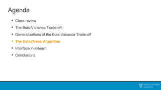
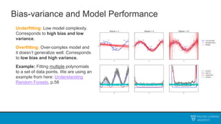
2 ⋅ (𝑓 𝑥 − 𝑓 𝑥 ) ⋅ 𝔼𝒟 𝑓 𝑥 − 𝑓𝒟 𝑥](https://image.slidesharecdn.com/mludtelecture2-230212190438-a3f17b7c/85/MLU_DTE_Lecture_2-pptx-25-320.jpg)
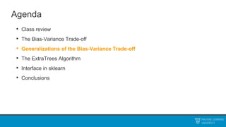
![Deriving the Relationship II
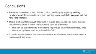
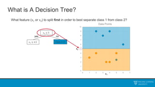
Now, let 𝑓(𝑥) = 𝔼𝒟[𝑓𝒟 𝑥 ] denote the average prediction of the ML model over every
training set. We may write:
𝔼𝒟 𝑓 𝑥 − 𝑓𝒟 𝑥
2
= 𝔼𝒟 𝑓 𝑥 − 𝑓 𝑥 + 𝑓 𝑥 − 𝑓𝒟 𝑥
2
= 𝔼𝒟 𝑓 𝑥 − 𝑓 𝑥
2
+ 𝔼𝒟 𝑓 𝑥 − 𝑓𝒟 𝑥
2
+2 ⋅ 𝔼𝑦,𝒟 𝑓 𝑥 − 𝑓 𝑥 𝑓 𝑥 − 𝑓𝒟 𝑥
Thus the last term is zero.
Also note 𝑓 𝑥 − 𝑓 𝑥 is not random, so the expectation does nothing on the left.
Doesn’t depend on
the dataset
Mean zero when
averaged over 𝒟
(2)
E 𝑋 + 𝑌 = 𝐸 𝑋 + 𝐸 𝑌
E 𝑎 𝑋 = 𝑎 𝐸 𝑋 , a: Constant
E 𝑋 𝑌 = 𝐸 𝑋 𝐸 𝑌 , X and Y are indep.
2 ⋅ (𝑓 𝑥 − 𝑓 𝑥 ) ⋅ 𝔼𝒟 𝑓 𝑥 − 𝑓𝒟 𝑥
2 ⋅ (𝑓 𝑥 − 𝑓 𝑥 ) ⋅ (𝔼𝒟 𝑓 𝑥 − 𝔼𝒟 𝑓𝒟 𝑥 )](https://image.slidesharecdn.com/mludtelecture2-230212190438-a3f17b7c/85/MLU_DTE_Lecture_2-pptx-26-320.jpg)
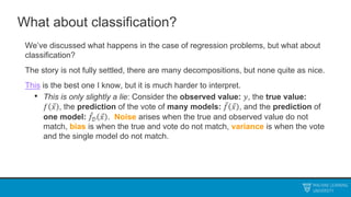
![Deriving the Relationship II
Now, let 𝑓(𝑥) = 𝔼𝒟[𝑓𝒟 𝑥 ] denote the average prediction of the ML model over every
training set. We may write:
𝔼𝒟 𝑓 𝑥 − 𝑓𝒟 𝑥
2
= 𝔼𝒟 𝑓 𝑥 − 𝑓 𝑥 + 𝑓 𝑥 − 𝑓𝒟 𝑥
2
= 𝔼𝒟 𝑓 𝑥 − 𝑓 𝑥
2
+ 𝔼𝒟 𝑓 𝑥 − 𝑓𝒟 𝑥
2
+2 ⋅ 𝔼𝑦,𝒟 𝑓 𝑥 − 𝑓 𝑥 𝑓 𝑥 − 𝑓𝒟 𝑥
Thus the last term is zero.
Also note 𝑓 𝑥 − 𝑓 𝑥 is not random, so the expectation does nothing on the left.
Doesn’t depend on
the dataset
Mean zero when
averaged over 𝒟
(2)
E 𝑋 + 𝑌 = 𝐸 𝑋 + 𝐸 𝑌
E 𝑎 𝑋 = 𝑎 𝐸 𝑋 , a: Constant
E 𝑋 𝑌 = 𝐸 𝑋 𝐸 𝑌 , X and Y are indep.
2 ⋅ (𝑓 𝑥 − 𝑓 𝑥 ) ⋅ 𝔼𝒟 𝑓 𝑥 − 𝑓𝒟 𝑥
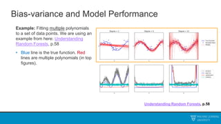
2 ⋅ (𝑓 𝑥 − 𝑓 𝑥 ) ⋅ (𝑓 𝑥 − 𝑓 𝑥 )
2 ⋅ (𝑓 𝑥 − 𝑓 𝑥 ) ⋅ (𝔼𝒟 𝑓 𝑥 − 𝔼𝒟 𝑓𝒟 𝑥 )
𝟎](https://image.slidesharecdn.com/mludtelecture2-230212190438-a3f17b7c/85/MLU_DTE_Lecture_2-pptx-27-320.jpg)
![Randomized Algorithms
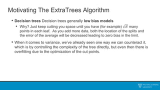
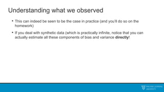
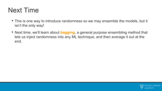
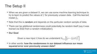
This generalization will be key to the entire rest of our class.
• Suppose that 𝑓𝒟 does not depend only on the data, but some additional
independent randomness that we add in ourselves, call it ℛ.
• If you follow through additional work, you can further decompose:
Var 𝑓𝒟 𝑥 = 𝔼𝒟 Varℛ 𝑓𝒟,ℛ 𝑥 |𝒟 + Var𝒟 𝔼ℛ 𝑓𝒟,ℛ 𝑥 |𝒟
• The first term is the average variance due to the added randomness, and the
second term is the variance in the average prediction due to the dataset.
𝑉𝑎𝑟 𝑌 = 𝐸[𝑉𝑎𝑟 𝑌 𝑋 ] + 𝑉𝑎𝑟(𝐸[𝑌|𝑋])](https://image.slidesharecdn.com/mludtelecture2-230212190438-a3f17b7c/85/MLU_DTE_Lecture_2-pptx-31-320.jpg)