Downloaded 464 times


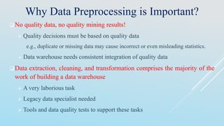
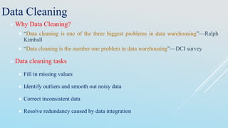


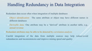

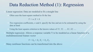
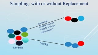
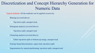
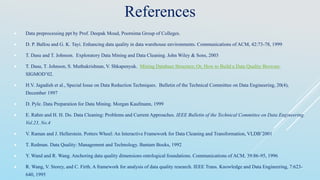
![Data Transformation: Normalization
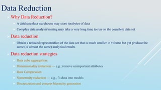
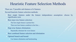
Min-max normalization: to [new_minA, new_maxA]
Ex. Let income range $12,000 to $98,000 normalized to [0.0, 1.0]. Then $73,000 is mapped to
Z-score normalization (μ: mean, σ: standard deviation):
Ex. Let μ = 54,000, σ = 16,000. Then
Normalization by decimal scaling
AAA
AA
A
minnewminnewmaxnew
minmax
minv
v _)__('
716.00)00.1(
000,12000,98
000,12600,73
A
Av
v
'
225.1
000,16
000,54600,73
j
v
v
10
' Where j is the smallest integer such that Max(|ν’|) < 1](https://image.slidesharecdn.com/datapreprocessing-150411051601-conversion-gate01/85/Data-preprocessing-25-320.jpg)


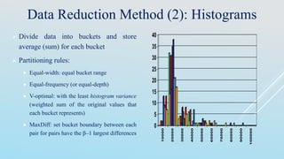

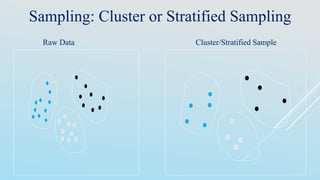

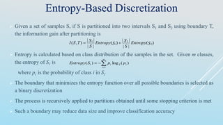
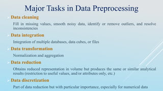
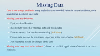
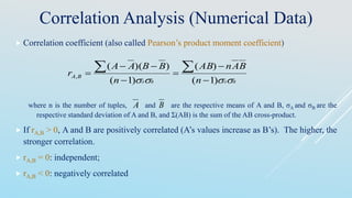
![Interval Merge by 2 Analysis
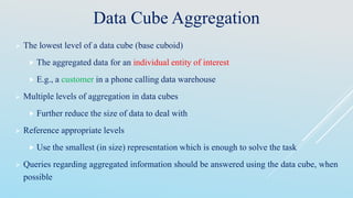
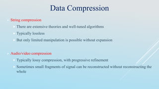
Merging-based (bottom-up) vs. splitting-based methods
Merge: Find the best neighboring intervals and merge them to form larger intervals
recursively
ChiMerge [Kerber AAAI 1992, See also Liu et al. DMKD 2002]
Initially, each distinct value of a numerical attr. A is considered to be one interval
2 tests are performed for every pair of adjacent intervals
Adjacent intervals with the lowest 2 values are merged together, since low 2 values
for a pair indicate similar class distributions
This merge process proceeds recursively until a predefined stopping criterion is met
(such as significance level, max-interval, max inconsistency, etc.)](https://image.slidesharecdn.com/datapreprocessing-150411051601-conversion-gate01/85/Data-preprocessing-48-320.jpg)
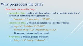
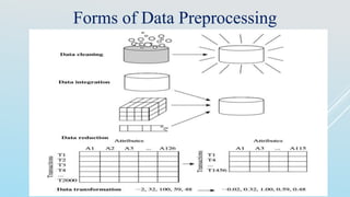
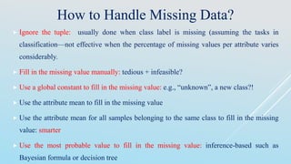
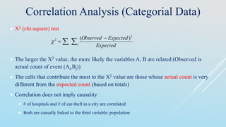
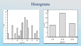
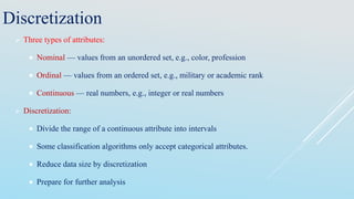
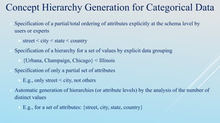
![Segmentation by Natural Partitioning
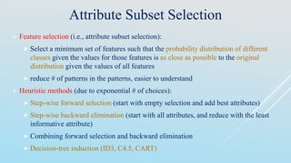
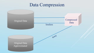
A simple 3-4-5 rule can be used to segment numeric data into relatively uniform,
“natural” intervals.
If an interval covers 3, 6, 7 or 9 distinct values at the most significant digit,
partition the range into 3 equi-width intervals (e.g. [12030, 81254] =>
[10000,80000] and 8-1 = 7 => 7 distinct values at the most significant digit)
If it covers 2, 4, or 8 distinct values at the most significant digit, partition the range
into 4 intervals
If it covers 1, 5, or 10 distinct values at the most significant digit, partition the
range into 5 intervals](https://image.slidesharecdn.com/datapreprocessing-150411051601-conversion-gate01/85/Data-preprocessing-49-320.jpg)

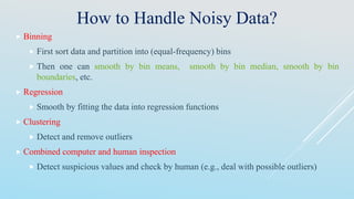
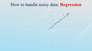
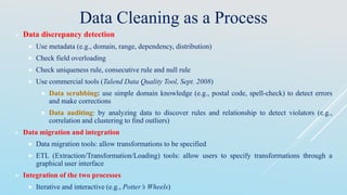
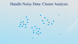
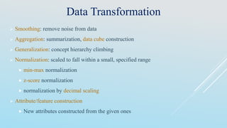
The document discusses data preprocessing techniques essential for data mining, highlighting the importance of addressing issues like incomplete, inconsistent, and noisy data. It outlines various tasks involved in data cleaning, integration, transformation, and reduction, emphasizing that quality data is crucial for effective mining results. Additionally, it reflects on different methods for handling missing and noisy data, as well as the need for correlation analysis and data normalization to maintain data integrity.