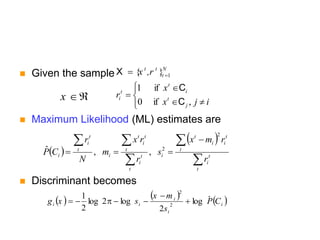
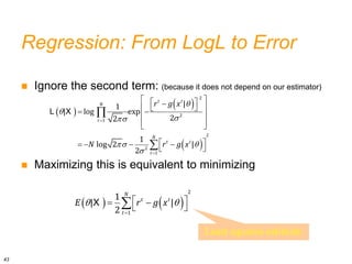
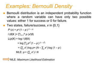
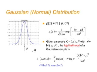
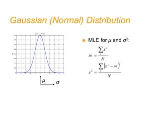
This document provides an overview of parametric methods in machine learning, including maximum likelihood estimation, evaluating estimators using bias and variance, the Bayes estimator, and parametric classification and regression. Key points covered include: - Maximum likelihood estimation chooses parameters that maximize the likelihood function to produce the most probable distribution given observed data. 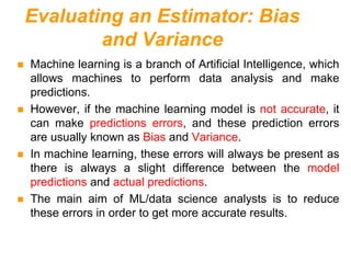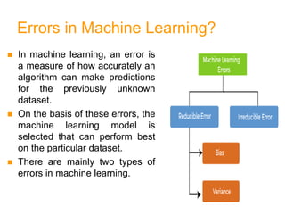- Bias and variance are used to evaluate estimators, with the goal of minimizing both to improve accuracy. High bias or variance can indicate underfitting or overfitting. 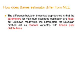- The Bayes estimator treats unknown parameters as random variables and uses prior distributions and Bayes' rule to estimate their expected values given data.

1. INTRODUCTION TO
Machine Learning
Lecture Slides for

2. CHAPTER 4:
Parametric Methods

3. Outline
 Introduction
 Maximum Likelihood Estimation
 Evaluating an Estimator: Bias and Variance
 The Bayes Estimator
 Parametric Classification
 Regression
 Tuning Model Complexity:
 Bias / Variance Dilemma
 Model Selection Procedures

4. Introduction
 A statistic is any value that is calculated from a given sample.
 In statistical inference, we make a decision using the
information provided by a sample.
 Our first approach is parametric where we assume that the
sample is drawn from some distribution that obeys a known
model, for example, Gaussian.
 The advantage of the parametric approach is that the model
is defined up to a small number of parameters—for example,
mean, variance—the sufficient statistics of the distribution.

5.  Once those parameters are estimated from the sample,
the whole distribution is known.
 We estimate the parameters of the distribution from the
given sample, plug in these estimates to the assumed
model, and get an estimated distribution, which we then
use to make a decision.
 The method we use to estimate the parameters of a
distribution is maximum likelihood estimation.
 We start with density estimation, which is the general case
of estimating p(x).
 We use this for classification where the estimated
densities are the class densities, p(x|Ci), and priors, P(Ci),
to be able to calculate the posteriors, P(Ci|x), and make
our decision.

6. Parametric Estimation
 X = { xt }t=1
N where xt ~ p(x)
 Here x is one dimensional and the densities are univariate.
 Parametric estimation:
Assume a form for p (x | θ) and estimate θ, its sufficient statistics,
using X
e.g., N ( μ, σ2) where θ = { μ, σ2}

7. Maximum Likelihood Estimation
 In statistics, maximum likelihood estimation (MLE) is a
method of estimating the parameters of an
assumed probability distribution, given some observed data.
 This is achieved by maximizing a likelihood function so that,
under the assumed statistical model, the observed data is
most probable.
 For example, if a population is known to follow a normal
distribution but the mean and variance are unknown.

8.  Let us say we have an independent and identically
distributed (iid) sample X = {xt}N
t=1.
 We assume that xt are instances drawn from some known
probability density family, p(x|θ), defined up to parameters,
θ:
 Likelihood of θ given the sample X
l (θ|X ) p(X |θ) = ∏ t=1
N p (xt|θ)
 Log likelihood
L(θ|X) log l (θ|X) = ∑ t=1
N log p (xt|θ)
 Maximum likelihood estimator (MLE)
θ* = arg maxθ L(θ|X)

9. Examples: Bernoulli Density
 Bernoulli distribution is an independent probability function
where a random variable can have only two possible
values: either 1 for success or 0 for failure.
 Two states, failure/success, x in {0,1}
P (x) = px (1 – p ) (1 – x)
l (θ|X )= ∏ t=1
N p (xt|θ)
L(p|X) = log l (θ|X)
= log ∏t
pxt
(1 – p ) (1 – xt)
= (∑t
xt ) log p+ (N – ∑t
xt ) log (1 – p )
MLE: p = (∑t
xt ) / N
MLE: Maximum Likelihood Estimation

10.  In probability theory and statistics, the Bernoulli
distribution, named after Swiss mathematician Jacob
Bernoulli, is the discrete probability distribution of
a random variable which takes the value 1 with
probability p and the value 0 with probability q=1-p.
 Less formally, it can be thought of as a model for the set
of possible outcomes of any single experiment that asks
a yes–no question.
 Such questions lead to outcomes that are boolean
valued: a single bit whose value is success / yes / true /
one with probability p and failure / no / false / zero with
probability q.

11.  It can be used to represent a (possibly biased) coin
toss where 1 and 0 would represent "heads" and "tails",
respectively, and p would be the probability of the coin
landing on heads (or vice versa where 1 would represent
tails and p would be the probability of tails).
 The Bernoulli distribution is a special case of the binomial
distribution where a single trial is conducted (so n would be
1 for such a binomial distribution).
 It is also a special case of the two-point distribution, for
which the possible outcomes need not be 0 and 1.

12. Examples: Multinomial Density
 K > 2 states, xi in {0,1}
P (x1,x2,...,xK) = ∏i
pi
xi
L(p1,p2,...,pK|X) = log ∏t
∏i
pi
xi
t
where xi
t = 1 if experiment t chooses state i
xi
t = 0 otherwise
MLE: pi = (∑t
xi
t ) / N
PS. K: mutually exclusive

13. Gaussian (Normal) Distribution
   











 2
2
2
exp
2
1 x
-
x
p
 p(x) = N ( μ, σ2)
 Given a sample X = { xt }t=1
N with xt ~
N ( μ, σ2) , the log likelihood of a
Gaussian sample is
μ σ
   












 2
2
2
exp
2
1 x
x
p
 
 
2
2
2
log
)
2
log(
2
|
,






 



 t
t
x
N
N
x
L
(Why? N samples?)

14. Gaussian (Normal) Distribution
   











 2
2
2
exp
2
1 x
-
x
p
 MLE for μ and σ2:
μ σ
 
N
m
x
s
N
x
m
t
t
t
t





2
2

15. Evaluating an Estimator: Bias
and Variance
 Machine learning is a branch of Artificial Intelligence, which
allows machines to perform data analysis and make
predictions.
 However, if the machine learning model is not accurate, it
can make predictions errors, and these prediction errors
are usually known as Bias and Variance.
 In machine learning, these errors will always be present as
there is always a slight difference between the model
predictions and actual predictions.
 The main aim of ML/data science analysts is to reduce
these errors in order to get more accurate results.

16. Errors in Machine Learning?
 In machine learning, an error is
a measure of how accurately an
algorithm can make predictions
for the previously unknown
dataset.
 On the basis of these errors, the
machine learning model is
selected that can perform best
on the particular dataset.
 There are mainly two types of
errors in machine learning.

17. What is Bias?
 In general, a machine learning model analyses the data,
find patterns in it and make predictions.
 While training, the model learns these patterns in the
dataset and applies them to test data for prediction.
 While making predictions, a difference occurs between
prediction values made by the model and actual
values/expected values, and this difference is known as
bias errors or Errors due to bias.

18. What is a Variance?
 The variance would specify the amount of variation in the
prediction if the different training data was used.
 In simple words, variance tells that how much a random
variable is different from its expected value.
 Ideally, a model should not vary too much from one training
dataset to another, which means the algorithm should be
good in understanding the hidden mapping between inputs
and output variables.
 Variance errors are either of low variance or high variance.

19. Different Combinations of Bias-Variance
19

20.  Low-Bias, Low-Variance: The combination of low bias and low
variance shows an ideal machine learning model. However, it is
not possible practically.
 Low-Bias, High-Variance: With low bias and high variance, model
predictions are inconsistent and accurate on average. This case
occurs when the model learns with a large number of parameters
and hence leads to an overfitting.
 High-Bias, Low-Variance: With High bias and low variance,
predictions are consistent but inaccurate on average. This case
occurs when a model does not learn well with the training dataset
or uses few numbers of the parameter. It leads
to underfitting problems in the model.
 High-Bias, High-Variance: With high bias and high variance,
predictions are inconsistent and also inaccurate on average.
Different Combinations of Bias-Variance

21. How to identify High variance or High Bias?
 High variance can be identified if the model has:
 Low training error and high test error.
 High Bias can be identified if the model has:
 High training error and the test error is almost similar to training
error.

22. Bias-Variance Trade-Off
 While building the machine learning model, it is really
important to take care of bias and variance in order to avoid
overfitting and underfitting in the model.
 If the model is very simple with fewer parameters, it may
have low variance and high bias.
 Whereas, if the model has a large number of parameters, it
will have high variance and low bias.
 So, it is required to make a balance between bias and
variance errors, and this balance between the bias error and
variance error is known as the Bias-Variance trade-off.

23.  For an accurate prediction of the model, algorithms need a
low variance and low bias.
 But this is not possible because bias and variance are
related to each other:
 If we decrease the variance, it will increase the bias.
 If we decrease the bias, it will increase the variance.
Hence, the Bias-
Variance trade-off
is about finding the
sweet spot to make
a balance between
bias and variance
errors.

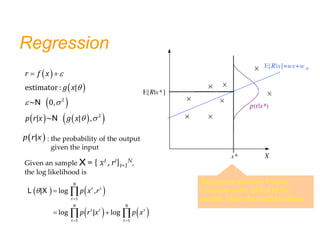
24. θ
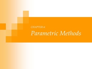
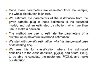
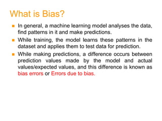
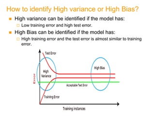
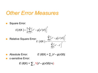
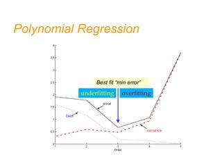
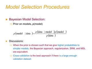
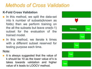
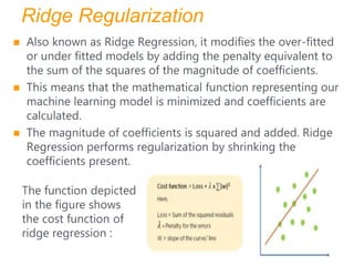
Bias and Variance
Unknown parameter θ
Estimator di = d (Xi)
on sample Xi
Bias: bθ(d) = E [d] – θ
Variance: E [(d–E [d])2]
If bθ(d) = 0
d is an unbiased estimator of θ
If E [(d–E [d])2] = 0
d is a consistent estimator of θ

25. Expected value
 If the probability distribution of X admits a probability density function f (x), then
the expected value can be computed as
 It follows directly from the discrete case definition that if X is a constant random
variable, i.e. X = b for some fixed real number b, then the expected value of X is
also b.
 The expected value of an arbitrary function of X, g(X), with respect to the
probability density function f(x) is given by the inner product of f and g:
http://en.wikipedia.org/wiki/Expected_value

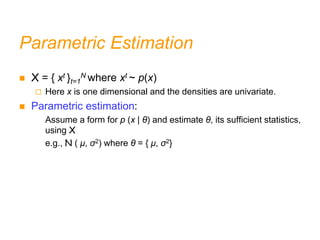
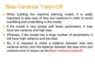
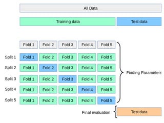
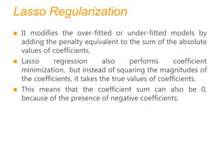
26. Bias and Variance
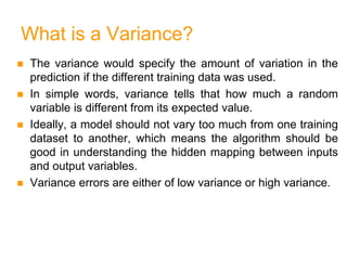
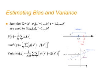
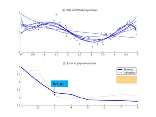
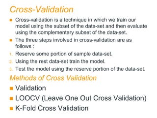
For example:
Var [m]  0 as N∞
m is also a consistent estimator
1
[ ] [ ]
t
t
t
t
x N
E m E E x
N N N


 
   
 
 
 


2 2
2 2
1
[ ] [ ]
t
t
t
t
x N
Var m Var Var x
N N N N
 
 
   
 
 
 



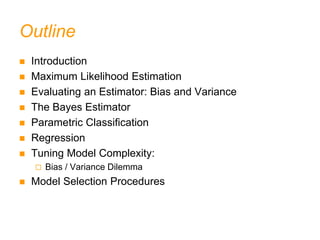
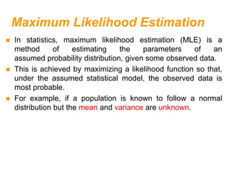
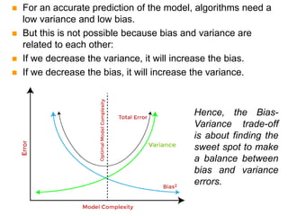
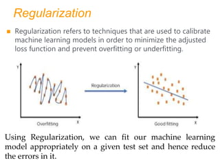
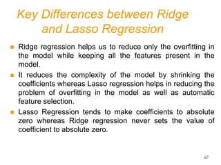
27. Bias and Variance
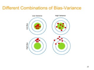
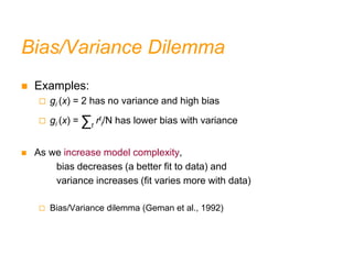
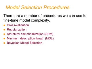
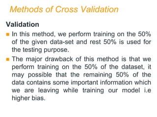
For example: (see P. 65-66)
s2 is a biased estimator of σ2
(N/(N-1))s2 is a unbiased estimator of σ2
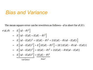
Mean square error:
r (d,θ) = E [(d–θ)2] (see P. 66, next slide)
= (E [d] – θ)2 + E [(d–E [d])2]
= Bias2 + Variance
2
2
2 1
)
( 
 





 

N
N
s
E
θ

28. Bias and Variance

29. Standard Deviation
 In statistics, the standard deviation is often estimated from a random
sample drawn from the population.
 The most common measure used is the sample standard deviation, which is
defined by
where is the sample (formally, realizations from a
random variable X) and is the sample mean.
http://en.wikipedia.org/wiki/Unbiased_estimation_of_standard_deviation
29

30. Bayes’ Estimator
 Sometimes, before looking at a sample, we (or experts of
the application) may have some prior information on the
possible value range that a parameter, θ, may take.
 This information is quite useful and should be used,
especially when the sample is small.
 The prior information does not tell us exactly what the
parameter value is (otherwise we would not need the
sample), and we model this uncertainty by viewing θ as a
random variable and by defining a prior density for it, p(θ).

31. What is a Bayesian estimator?
 A Bayesian estimator is an estimator of an
unknown parameter θ that minimizes the expected loss
for all observations x of X.
 An estimator is Bayesian if it uses the Bayes theorem to
predict the most likely class of some observed data.
 Because the class of data is an unknown parameter and
not a random variable, it is not possible to express the
probability of that class using the standard concept of
probability.

32. How does Bayes estimator differ from MLE
 The difference between these two approaches is that the
parameters for maximum likelihood estimation are fixed,
but unknown meanwhile the parameters for Bayesian
method act as random variables with known prior
distributions

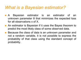
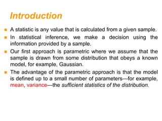
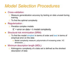
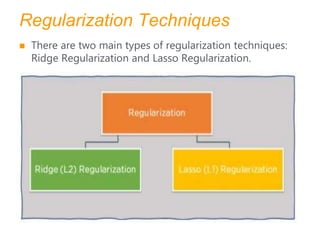
33. Bayes’ Estimator
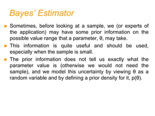
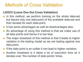
 Treat θ as a random variable with prior p(θ)
 Bayes’ rule:
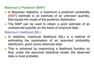
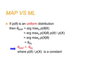
 Maximum a Posteriori (MAP):
θMAP = arg maxθ p(θ|X)
 Maximum Likelihood (ML):
θML = arg maxθ p(X|θ)
 Bayes’ estimator:
θBayes = E[θ|X] = ∫ θ p(θ|X) dθ
( | ) ( )
( | )
( )
p X p
p X
p X
 
 

34. Maximum a Posteriori (MAP):
 In Bayesian statistics, a maximum a posteriori probability
(MAP) estimate is an estimate of an unknown quantity,
that equals the mode of the posterior distribution.
 The MAP can be used to obtain a point estimate of an
unobserved quantity on the basis of empirical data.
Maximum Likelihood (ML):
 In statistics, maximum likelihood (ML) is a method of
estimating the parameters of an assumed probability
distribution, given some observed data.
 This is achieved by maximizing a likelihood function so
that, under the assumed statistical model, the observed
data is most probable.

35. MAP VS ML
 If p(θ) is an uniform distribution
then θMAP = arg maxθ p(θ|X)
= arg maxθ p(X|θ) p(θ) / p(X)
= arg maxθ p(X|θ)
= θML
θMAP = θML
where p(θ) / p(X) is a constant

36. Bayes’ Estimator: Example
 If p (θ|X) is normal, then θML = m and θBayes =θMAP
 Example: Suppose xt ~ N (θ, σ2) and θ ~ N ( μ0, σ0
2)
θBayes =
 The Bayes’ estimator is a weighted average of the prior mean μ0 and the
sample mean m.
 
2
2
0
0
2 2 2 2
0 0
1/
/
|
/ 1/ / 1/
N
E m
N N


 
   
 
 
X
 
2
1
/2 2
( )
1
| exp[ ]
(2 ) 2
N
t
t
N N
x
p


  


 

X
 
 
2
0
2
0
0
1
exp
2
2
p
 



 

 
 
 
 
θML = m
36

37. Parametric Classification
 The discriminant function
 Assume that are Gaussian
     
     
i
i
i
i
i
i
C
P
C
x
p
x
g
C
P
C
x
p
x
g
log
|
log
ly
equivalent
or
|



   
     
i
i
i
i
i
i
i
i
i
C
P
x
x
g
x
C
x
p
log
2
log
2
log
2
1
2
exp
2
1
|
2
2
2
2























 
i
C
x
p |
37
log likelihood of a Gaussian sample

38.  Given the sample
 Maximum Likelihood (ML) estimates are
 Discriminant becomes
N
t
t
t
,r
x 1
}
{ 

X


x 








,
if
0
if
1
i
j
x
x
r
j
t
i
t
t
i
C
C
 
 




 



t
t
i
t
t
i
i
t
i
t
t
i
t
t
i
t
i
t
t
i
i
r
r
m
x
s
r
r
x
m
N
r
C
P
2
2
,
,
ˆ
     
i
i
i
i
i C
P̂
s
m
x
s
x
g log
2
log
2
log
2
1
2
2








39.  The first term is a constant and if the priors are equal,
those terms can be dropped.
 Assume that variances are equal, then
becomes
Choose Ci if
 
 
 
2
2
1 ˆ
log 2 log log
2 2
i
i i i
i
x m
g x s P C
s


    
   
2
i i
g x x m
  
|
|
min
|
| k
k
i m
x
m
x 



40. Equal
variances
Single boundary at
halfway between
means
Likelihood functions and the posteriors with equal priors for two classes when the input is one-dimensional.
Variances are equal and the posteriors intersect at one point, which is the threshold of decision.

41. Variances are
different
Two boundaries
Likelihood functions and the posteriors with equal priors for two classes when the input is one-dimensional.
Variances are unequal and the posteriors intersect at two points.

42. Regression
 
 
 
   
 


 
 
 
N ,
N ,
2
2
estimator: |
~ 0
| ~ |
r f x
g x
p r x g x
   
   


 

 

 
L X
1
1 1
| log ,
log | log
N
t t
t
N N
t t t
t t
p x r
p r x p x
Regression assumes 0 mean
Gaussian noise added to the
model; Here, the model is linear.
 
|
p r x : the probability of the output
given the input
Given an sample X = { xt , rt}t=1
N,
the log likelihood is

43. Regression: From LogL to Error
 Ignore the second term: (because it does not depend on our estimator)
 Maximizing this is equivalent to minimizing
 
 
 




 



 
 

 
 
 
 
 
 
 
   
 


L X
2
2
1
2
2
1
|
1
| log exp
2
2
1
log 2 |
2
t t
N
t
N
t t
t
r g x
N r g x
   
 

 
 
 

X
2
1
1
| |
2
N
t t
t
E r g x
Least squares estimate
43

44. Example: Linear Regression
  
1 0 1 0
Let | ,
t t
g x w w w x w
 
 
 
 
  
0 1
2
0 1
We can obtain
and
t t
t t
t t t t
t t t
r Nw w x
r x w x w x
 
   
     
  
     
 
   
 
 
 

 
0
2
1
, ,
t t
t t
t t
t t
t
t t
N x r
w
w r x
x x
w y
A 
 1
w y
A
(Exercise!!)
   
 

 
 
 

X
2
1
1
Minimize | |
2
N
t t
t
E r g x
44
Aw = y

45. Example: Polynomial Regression
     
    
2
2 1 0 2 1 0
| ,..., , , ...
k
t t t t
k k
g x w w w w w x w x w x w
   
   
   
 
   
   
   
 
   
   
 
   
 
 
2
1 1 1
1
2
2
2 2 2
2 2
1 ...
1 ...
Let ,
:
:
1 ...
k
k
N
N N N
x x x
r
r
x x x
r
x x x
r
D
 

We can obtain ,
T
A D D  


1
T T
w r
D D D
 
 , and
T
y D r
45
(see page 75)
Aw = y

46. Other Error Measures
 Square Error:
 Relative Square Error:
 Absolute Error: E (θ|X) = ∑t
|rt – g(xt|θ)|
 ε-sensitive Error:
E (θ|X) = ∑t
1(|rt – g(xt|θ)|>ε)
   
 

 
 
 

X
2
1
1
| |
2
N
t t
t
E r g x
 
 

 

 

 

 

 


X
2
1
2
1
|
|
N
t t
t
N
t
t
r g x
E
r r

47. Bias and Variance
(See Eq. 4.17)
Now let’s note that g(.) is a random variable (function) of samples S:
The expected square error at a particular point x wrt
to a fixed g(x) and variations in r based on p(r|x):
E[(r-g(x))2
|x]=E[(r-E[r|x])2
|x]+(E[r|x]- g(x))2
noise squared error
ES
[E[(r- g(x))2
|x]]=E[(r-E[r|x])2
|x]+ES
[(E[r|x]- g(x))2
]
Estimate for
the error at
point x
Expectation of our estimate for
the error at point x (wrt sample
variation)

48. Bias and Variance
ES
[(E[r|x]- g(x))2
|x]=
(E[r|x]-ES
[g(x)])2
+ES
[(g(x)-ES
[g(x)])2
]
bias2 variance
The expected value (average over samples X, all of size N and
drawn from the same joint density p(x, r)) : (See Eq. 4.11)
(See page 66 and 76)
squared error
squared error = bais2+variance
Now let’s note that g(.) is a random variable (function) of samples S:
ES
[E[(r- g(x))2
|x]]=E[(r-E[r|x])2
|x]+ES
[(E[r|x]- g(x))2
]

49. Estimating Bias and Variance
 Samples Xi={xt
i , rt
i}, i =1,...,M, t = 1,2,…,N
are used to fit gi (x), i =1,...,M
   
     
     

 
 
 
 
 
 



2
2
2
1
1
Bias
1
Variance
i
i
t t
t
t t
i
t i
g x g x
M
g g x f x
N
g g x g x
NM
θ

50. Bias/Variance Dilemma
 Examples:
 gi (x) = 2 has no variance and high bias
 gi (x) = ∑t
rt
i/N has lower bias with variance
 As we increase model complexity,
bias decreases (a better fit to data) and
variance increases (fit varies more with data)
 Bias/Variance dilemma (Geman et al., 1992)

51. bias
f
gi g
f
)
5
.
1
sin(
2
)
( x
x
f 
variance

52. Polynomial Regression
Best fit “min error”
overfitting
underfitting

53. Best fit,
Fig. 4.7

54. Model Selection Procedures
There are a number of procedures we can use to
fine-tune model complexity.
 Cross-validation
 Regularization
 Structural risk minimization (SRM)
 Minimum description length (MDL)
 Bayesian Model Selection

55. Model Selection Procedures
 Cross-validation:
 Measure generalization accuracy by testing on data unused during
training
 To find the optimal complexity
 Regularization :
 Penalize complex models
E’ = error on data + λ model complexity
 Structural risk minimization (SRM):
 To find the model simplest in terms of order and best in terms of
empirical error on the data
 Model complexity measure: polynomials of increasing order, VC
dimension, ...
 Minimum description length (MDL):
 Kolmogorov complexity of a data set is defined as the shortest
description of data

56. Model Selection Procedures
 Bayesian Model Selection:
 Prior on models, p(model)
 Discussions:
 When the prior is chosen such that we give higher probabilities to
simpler models, the Bayesian approach, regularization, SRM, and MDL
are equivalent.
 Cross-validation is the best approach if there is a large enough
validation dataset.
     
 
data
model
model
|
data
data
|
model
p
p
p
p 

57. Cross-Validation
 Cross-validation is a technique in which we train our
model using the subset of the data-set and then evaluate
using the complementary subset of the data-set.
 The three steps involved in cross-validation are as
follows :
1. Reserve some portion of sample data-set.
2. Using the rest data-set train the model.
3. Test the model using the reserve portion of the data-set.
Methods of Cross Validation
 Validation
 LOOCV (Leave One Out Cross Validation)
 K-Fold Cross Validation

58. Methods of Cross Validation
Validation
 In this method, we perform training on the 50%
of the given data-set and rest 50% is used for
the testing purpose.
 The major drawback of this method is that we
perform training on the 50% of the dataset, it
may possible that the remaining 50% of the
data contains some important information which
we are leaving while training our model i.e
higher bias.

59. Methods of Cross Validation
LOOCV (Leave One Out Cross Validation)
 In this method, we perform training on the whole data-set
but leaves only one data-point of the available data-set and
then iterates for each data-point.
 It has some advantages as well as disadvantages also.
 An advantage of using this method is that we make use of
all data points and hence it is low bias.
 The major drawback of this method is that it leads to higher
variation in the testing model as we are testing against one
data point.
 If the data point is an outlier it can lead to higher variation.
 Another drawback is it takes a lot of execution time as it
iterates over ‘the number of data points’ times.

60. Methods of Cross Validation
K-Fold Cross Validation
 In this method, we split the data-set
into k number of subsets(known as
folds) then we perform training on
the all the subsets but leave one(k-1)
subset for the evaluation of the
trained model.
 In this method, we iterate k times
with a different subset reserved for
testing purpose each time.
Note:
 It is always suggested that the value of
k should be 10 as the lower value of k is
takes towards validation and higher
value of k leads to LOOCV method.

62. Regularization
 Regularization refers to techniques that are used to calibrate
machine learning models in order to minimize the adjusted
loss function and prevent overfitting or underfitting.
Using Regularization, we can fit our machine learning
model appropriately on a given test set and hence reduce
the errors in it.

63. Regularization Techniques
 There are two main types of regularization techniques:
Ridge Regularization and Lasso Regularization.

64. Ridge Regularization
 Also known as Ridge Regression, it modifies the over-fitted
or under fitted models by adding the penalty equivalent to
the sum of the squares of the magnitude of coefficients.
 This means that the mathematical function representing our
machine learning model is minimized and coefficients are
calculated.
 The magnitude of coefficients is squared and added. Ridge
Regression performs regularization by shrinking the
coefficients present.
The function depicted
in the figure shows
the cost function of
ridge regression :

65. Lasso Regularization
 It modifies the over-fitted or under-fitted models by
adding the penalty equivalent to the sum of the absolute
values of coefficients.
 Lasso regression also performs coefficient
minimization, but instead of squaring the magnitudes of
the coefficients, it takes the true values of coefficients.
 This means that the coefficient sum can also be 0,
because of the presence of negative coefficients.

66. Key Differences between Ridge
and Lasso Regression
 Ridge regression helps us to reduce only the overfitting in
the model while keeping all the features present in the
model.
 It reduces the complexity of the model by shrinking the
coefficients whereas Lasso regression helps in reducing the
problem of overfitting in the model as well as automatic
feature selection.
 Lasso Regression tends to make coefficients to absolute
zero whereas Ridge regression never sets the value of
coefficient to absolute zero.
67