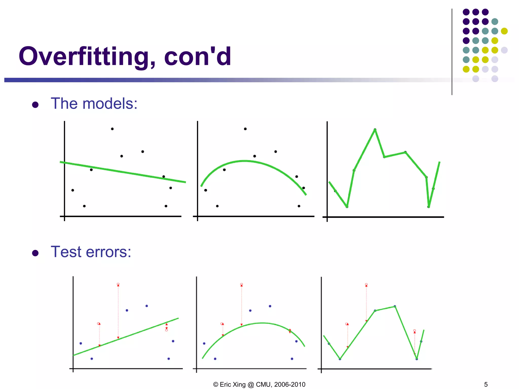
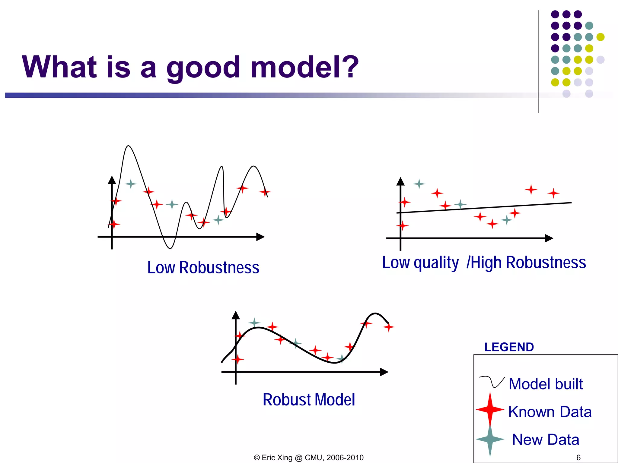
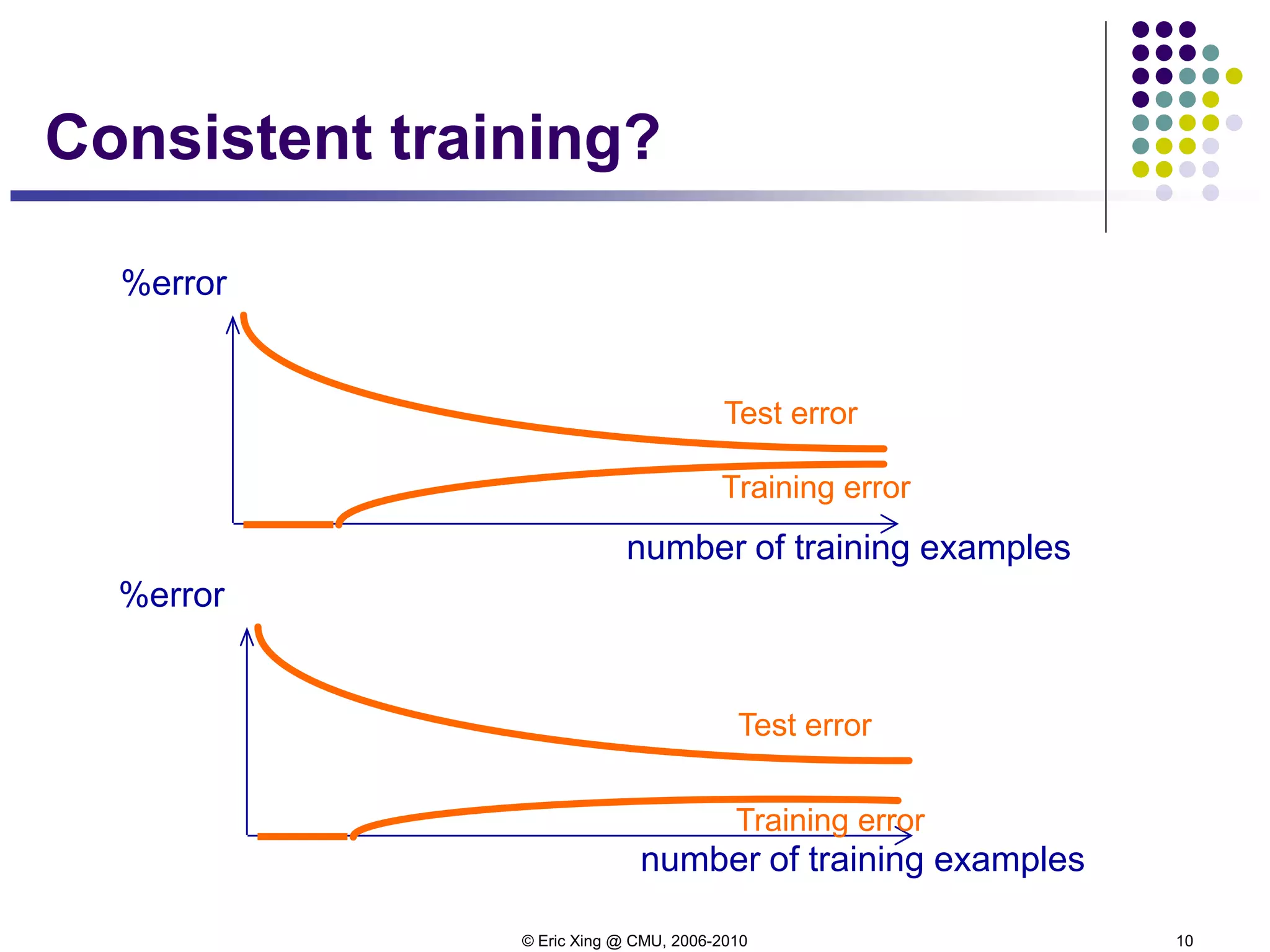
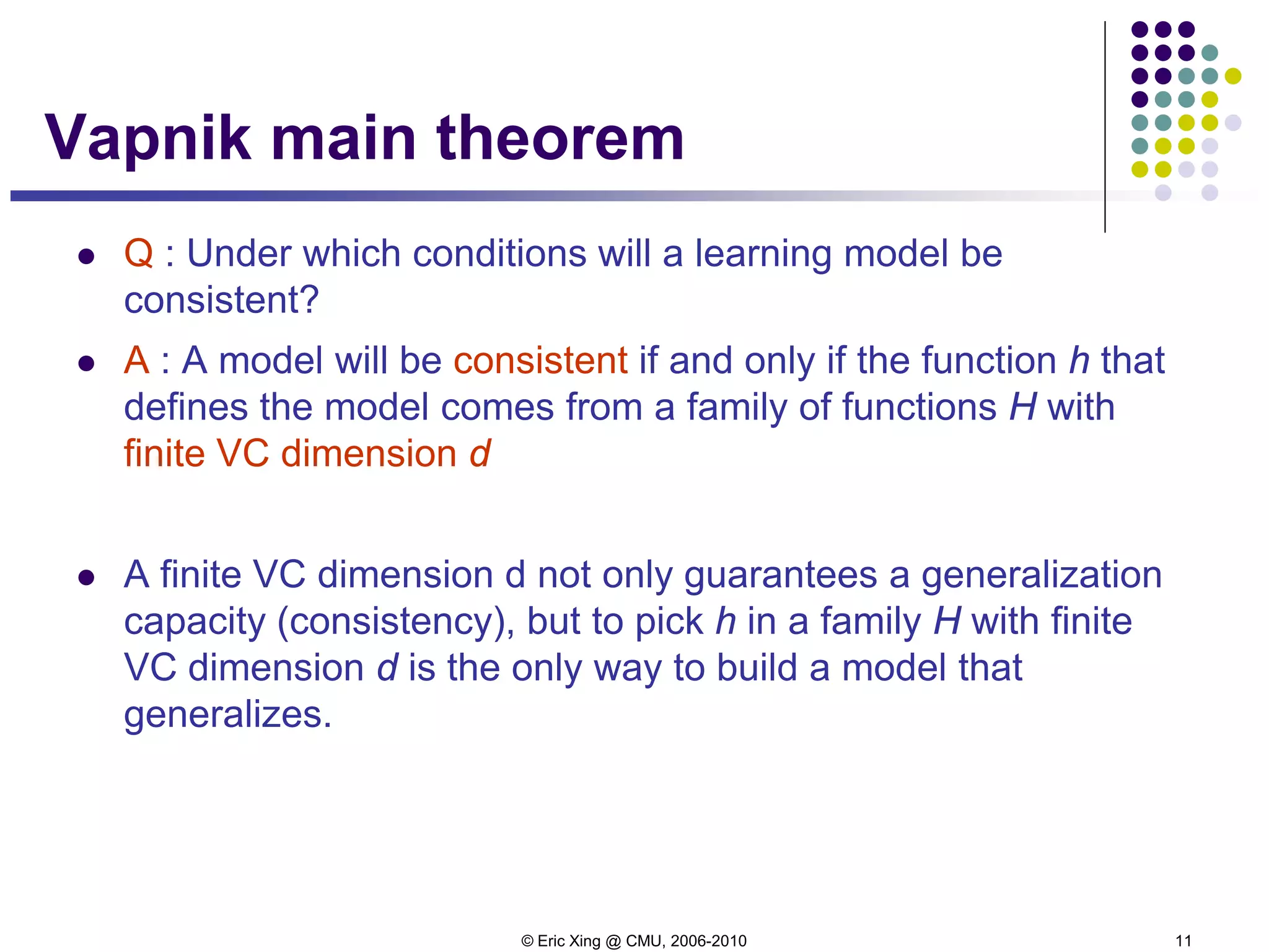
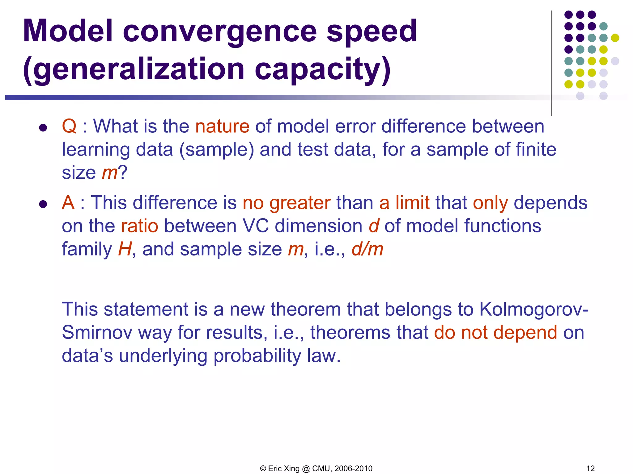
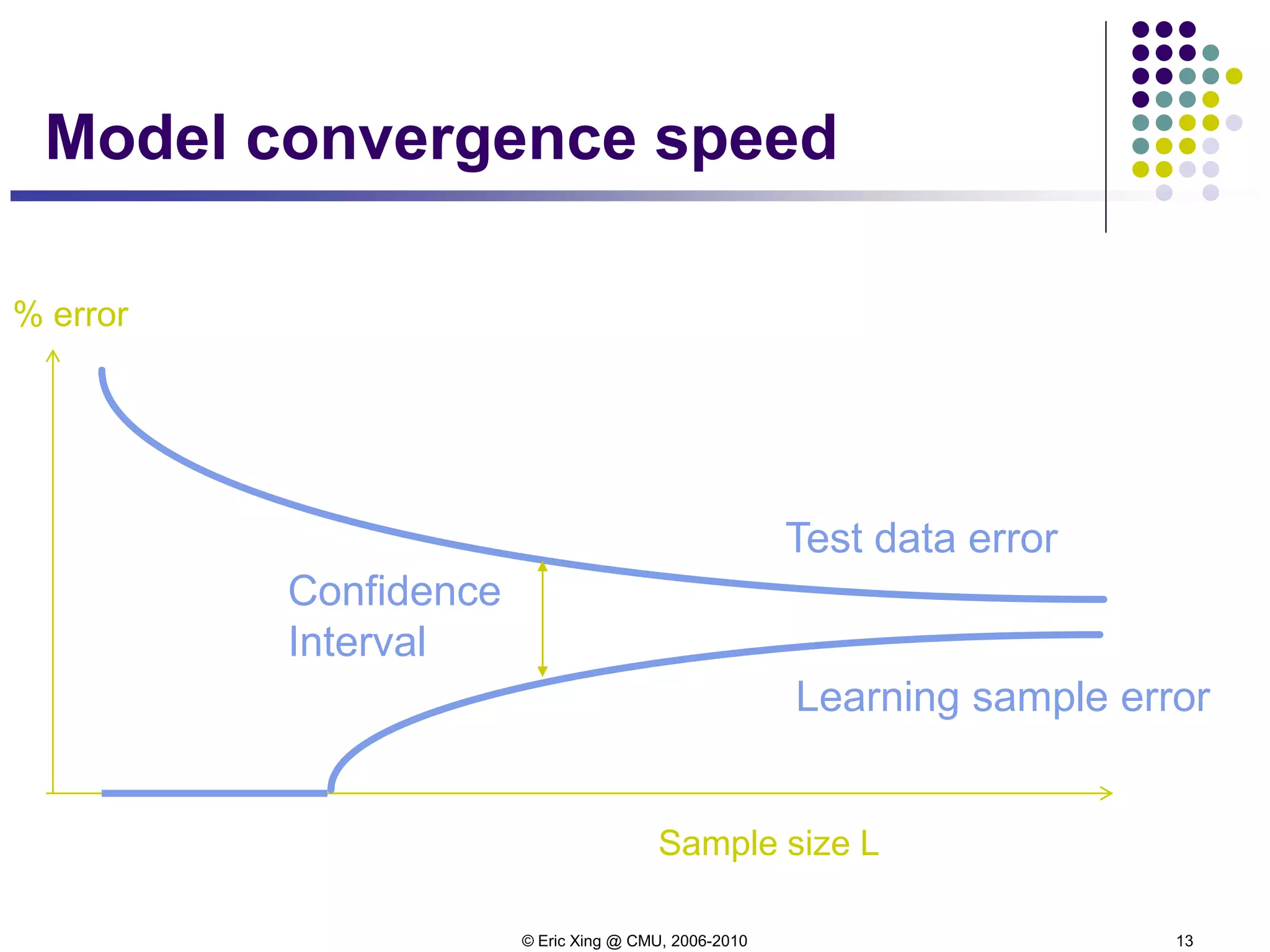
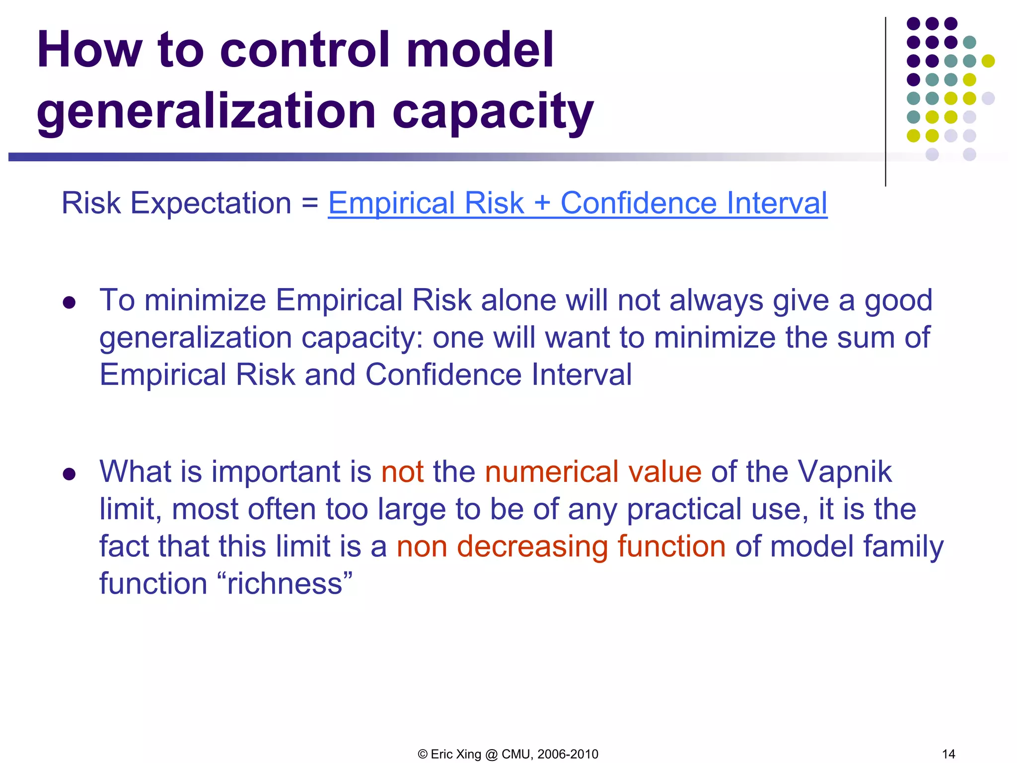
This document provides an overview of machine learning concepts related to overfitting and model selection. It discusses overfitting in k-nearest neighbors and regression models. It introduces bias-variance decomposition and structural risk minimization. Methods for controlling overfitting like cross-validation, regularization, feature selection and model selection are covered. The concepts of consistency, model convergence speed, and strategies for controlling generalization capacity are explained.

1. © Eric Xing @ CMU, 2006-2010 1
Machine Learning
Overfitting and Model Selection
Eric Xing
Lecture 6, August 13, 2010
Reading:

2. © Eric Xing @ CMU, 2006-2010 2
Outline
 Overfitting
 kNN
 Regression
 Bias-variance decomposition
 Generalization Theory and Structural Risk Minimization
 The battle against overfitting:
each learning algorithm has some "free knobs" that one can "tune" (i.e.,
heck) to make the algorithm generalizes better to test data.
But is there a more principled way?
 Cross validation
 Regularization
 Feature selection
 Model selection --- Occam's razor
 Model averaging

3. © Eric Xing @ CMU, 2006-2010 3
Overfitting: kNN

4. © Eric Xing @ CMU, 2006-2010 4
Another example:
 Regression

5. © Eric Xing @ CMU, 2006-2010 5
Overfitting, con'd
 The models:
 Test errors:

6. © Eric Xing @ CMU, 2006-2010 6
What is a good model?
Low Robustness
Robust Model
Low quality /High Robustness
Model built
Known Data
New Data
LEGEND

7. © Eric Xing @ CMU, 2006-2010 7
Bias-variance decomposition
 Now let's look more closely into two sources of errors in an
functional approximator:
 Let h(x) = E[t|x] be the optimal predictor, and y(x) our actual
predictor:
 expected loss = (bias)2 + variance + noise
( )[ ] [ ]( ) [ ]( )[ ]222
);();()();()();( DxyEDxyExhDxyExhDxyE DDDD −+−=−

8. © Eric Xing @ CMU, 2006-2010 8
Four Pillars for SLT
 Consistency (guarantees generalization)
 Under what conditions will a model be consistent ?
 Model convergence speed (a measure for generalization)
 How does generalization capacity improve when sample size L grows?
 Generalization capacity control
 How to control in an efficient way model generalization starting with the only given
information we have: our sample data?
 A strategy for good learning algorithms
 Is there a strategy that guarantees, measures and controls our learning model
generalization capacity ?

9. © Eric Xing @ CMU, 2006-2010 10
%error
number of training examples
Test error
Training error
%error
number of training examples
Test error
Training error
Consistent training?

10. © Eric Xing @ CMU, 2006-2010 11
 Q : Under which conditions will a learning model be
consistent?
 A : A model will be consistent if and only if the function h that
defines the model comes from a family of functions H with
finite VC dimension d
 A finite VC dimension d not only guarantees a generalization
capacity (consistency), but to pick h in a family H with finite
VC dimension d is the only way to build a model that
generalizes.
Vapnik main theorem

11. © Eric Xing @ CMU, 2006-2010 12
Model convergence speed
(generalization capacity)
 Q : What is the nature of model error difference between
learning data (sample) and test data, for a sample of finite
size m?
 A : This difference is no greater than a limit that only depends
on the ratio between VC dimension d of model functions
family H, and sample size m, i.e., d/m
This statement is a new theorem that belongs to Kolmogorov-
Smirnov way for results, i.e., theorems that do not depend on
data’s underlying probability law.

12. © Eric Xing @ CMU, 2006-2010 13
Sample size L
Confidence
Interval
Test data error
Learning sample error
% error
Model convergence speed

13. © Eric Xing @ CMU, 2006-2010 14
How to control model
generalization capacity
Risk Expectation = Empirical Risk + Confidence Interval
 To minimize Empirical Risk alone will not always give a good
generalization capacity: one will want to minimize the sum of
Empirical Risk and Confidence Interval
 What is important is not the numerical value of the Vapnik
limit, most often too large to be of any practical use, it is the
fact that this limit is a non decreasing function of model family
function “richness”

14. © Eric Xing @ CMU, 2006-2010 15
 With probability 1-δ, the following inequality is true:
 where w0 is the parameter w value that minimizes Empirical Risk:
Empirical Risk Minimization

15. © Eric Xing @ CMU, 2006-2010 16
Structural Risk Minimization
 Which hypothesis space should we choose?
 Bias / variance tradeoff
 SRM: choose H to minimize bound on true error!
unfortunately a somewhat loose bound...

16. © Eric Xing @ CMU, 2006-2010 17
SRM strategy (1)
 With probability 1-δ,
 When m/d is small (d too large), second term of equation becomes
large
 SRM basic idea for strategy is to minimize simultaneously both
terms standing on the right of above majoring equation for ε(h)
 To do this, one has to make d a controlled parameter

17. © Eric Xing @ CMU, 2006-2010 18
SRM strategy (2)
 Let us consider a sequence H1 < H2 < .. < Hn of model family
functions, with respective growing VC dimensions
d1 < d2 < .. < dn
 For each family Hi of our sequence, the inequality
is valid
 That is, for each subset, we must be able either to compute d, or to get a bound
on d itself.
 SRM then consists of finding that subset of functions which
minimizes the bound on the actual risk.

18. © Eric Xing @ CMU, 2006-2010 19
SRM : find i such that expected risk ε(h) becomes
minimum, for a specific d*=di, relating to a specific
family Hi of our sequence; build model using h from Hi
Empirical
Risk
Risk
Model Complexity
Total Risk
Confidence interval
In h/L
Best Model
h*
SRM strategy (3)

19. © Eric Xing @ CMU, 2006-2010 20
Putting SRM into action:
linear models case (1)
 There are many SRM-based strategies to build models:
 In the case of linear models
y = wTx + b,
one wants to make ||w|| a controlled parameter: let us call HC the
linear model function family satisfying the constraint:
||w|| < C
Vapnik Major theorem:
When C decreases, d(HC) decreases
||x|| < R

20. © Eric Xing @ CMU, 2006-2010 21
Putting SRM into action:
linear models case (2)
 To control ||w||, one can envision two routes to model:
 Regularization/Ridge Regression, ie min. over w and b
RG(w,b) = S{(yi-<w|xi> - b)² |i=1,..,L} + λ ||w||²
 Support Vector Machines (SVM), ie solve directly an optimization
problem (classif. SVM, separable data)
Minimize ||w||²,
with (yi= +/-1)
and yi(<w|xi> + b) >=1 for all i=1,..,L

21. © Eric Xing @ CMU, 2006-2010 22
Regularized Regression
 Recall linear regression:
 Regularized LR:
 L2-regularized LR:
 L1-regularized LR:

22. © Eric Xing @ CMU, 2006-2010 23
Bias-variance tradeoff
 λ is a "regularization"
terms in LR, the smaller
the λ, is more complex the
model (why?)
 Simple (highly regularized)
models have low variance but
high bias.
 Complex models have low bias
but high variance.
 You are inspecting an
empirical average over
100 training set.
 The actual ED can not be
computed

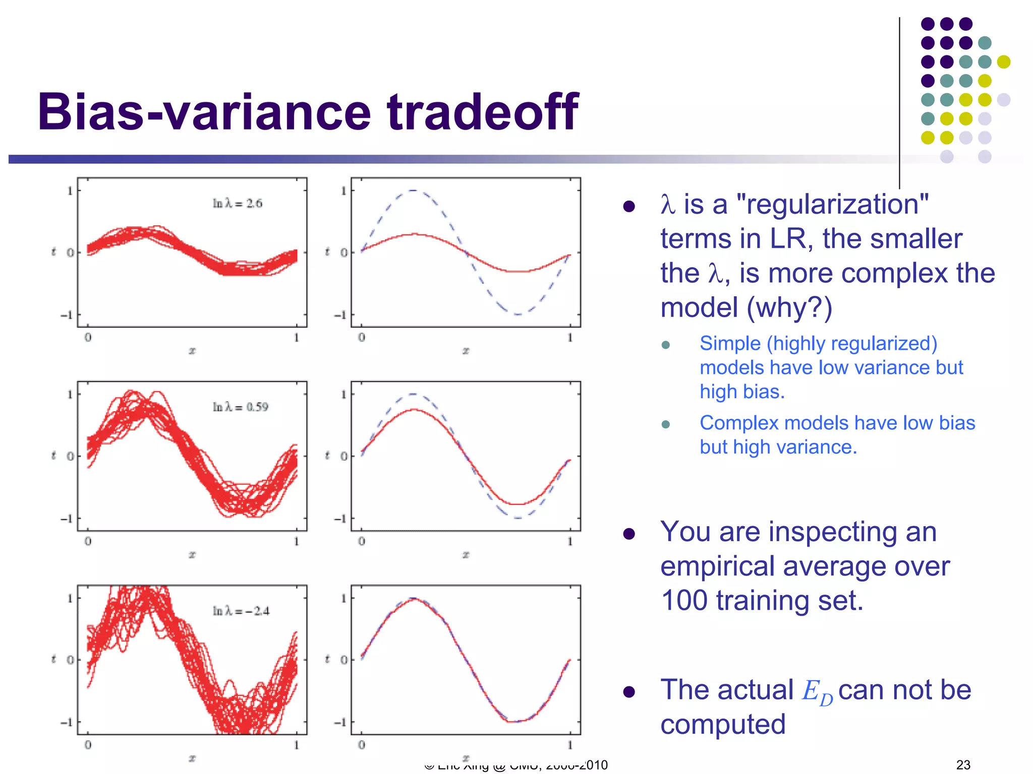
23. © Eric Xing @ CMU, 2006-2010 24
Bias2+variance vs regularizer
 Bias2+variance predicts (shape of) test error quite well.
 However, bias and variance cannot be computed since it
relies on knowing the true distribution of x and t (and hence
h(x) = E[t|x]).

24. © Eric Xing @ CMU, 2006-2010 25
The battle against overfitting

25. © Eric Xing @ CMU, 2006-2010 26
Model Selection
 Suppose we are trying select among several different models
for a learning problem.
 Examples:
1. polynomial regression
 Model selection: we wish to automatically and objectively decide if k should be, say, 0,
1, . . . , or 10.
2. locally weighted regression,
 Model selection: we want to automatically choose the bandwidth parameter τ.
3. Mixture models and hidden Markov model,
 Model selection: we want to decide the number of hidden states
 The Problem:
 Given model family , find s.t.
)();( k
k xxxgxh θθθθθ ++++= 2
210
{ }IMMM ,,, 21=F F∈iM
),(maxarg MDJM
M
i
F∈
=

26. © Eric Xing @ CMU, 2006-2010 27
1. Cross Validation
 We are given training data D and test data Dtest, and we would
like to fit this data with a model pi(x;θ) from the family F (e.g,
an LR), which is indexed by i and parameterized by θ.
 K-fold cross-validation (CV)
 Set aside αN samples of D (where N = |D|). This is known as the held-out data
and will be used to evaluate different values of i.
 For each candidate model i, fit the optimal hypothesis pi(x;θ∗) to the remaining
(1−α)N samples in D (i.e., hold i fixed and find the best θ).
 Evaluate each model pi(x|θ∗) on the held-out data using some pre-specified risk
function.
 Repeat the above K times, choosing a different held-out data set each time, and
the scores are averaged for each model pi(.) over all held-out data set. This gives
an estimate of the risk curve of models over different i.
 For the model with the lowest risk, say pi*(.), we use all of D to find the
parameter values for pi*(x;θ∗).

27. © Eric Xing @ CMU, 2006-2010 28
Example:
 When α=1/N, the algorithm is known as Leave-One-Out-
Cross-Validation (LOOCV)
MSELOOCV(M2)=0.962MSELOOCV(M1)=2.12

28. © Eric Xing @ CMU, 2006-2010 29
Practical issues for CV
 How to decide the values for K and α
 Commonly used K = 10 and α = 0.1.
 when data sets are small relative to the number of models that are being
evaluated, we need to decrease α and increase K
 K needs to be large for the variance to be small enough, but this makes it time-
consuming.
 Bias-variance trade-off
 Small α usually lead to low bias. In principle, LOOCV provides an almost
unbiased estimate of the generalization ability of a classifier, especially when the
number of the available training samples is severely limited; but it can also have
high variance.
 Large α can reduce variance, but will lead to under-use of data, and causing high-
bias.
 One important point is that the test data Dtest is never used in
CV, because doing so would result in overly (indeed
dishonest) optimistic accuracy rates during the testing phase.

29. © Eric Xing @ CMU, 2006-2010 30
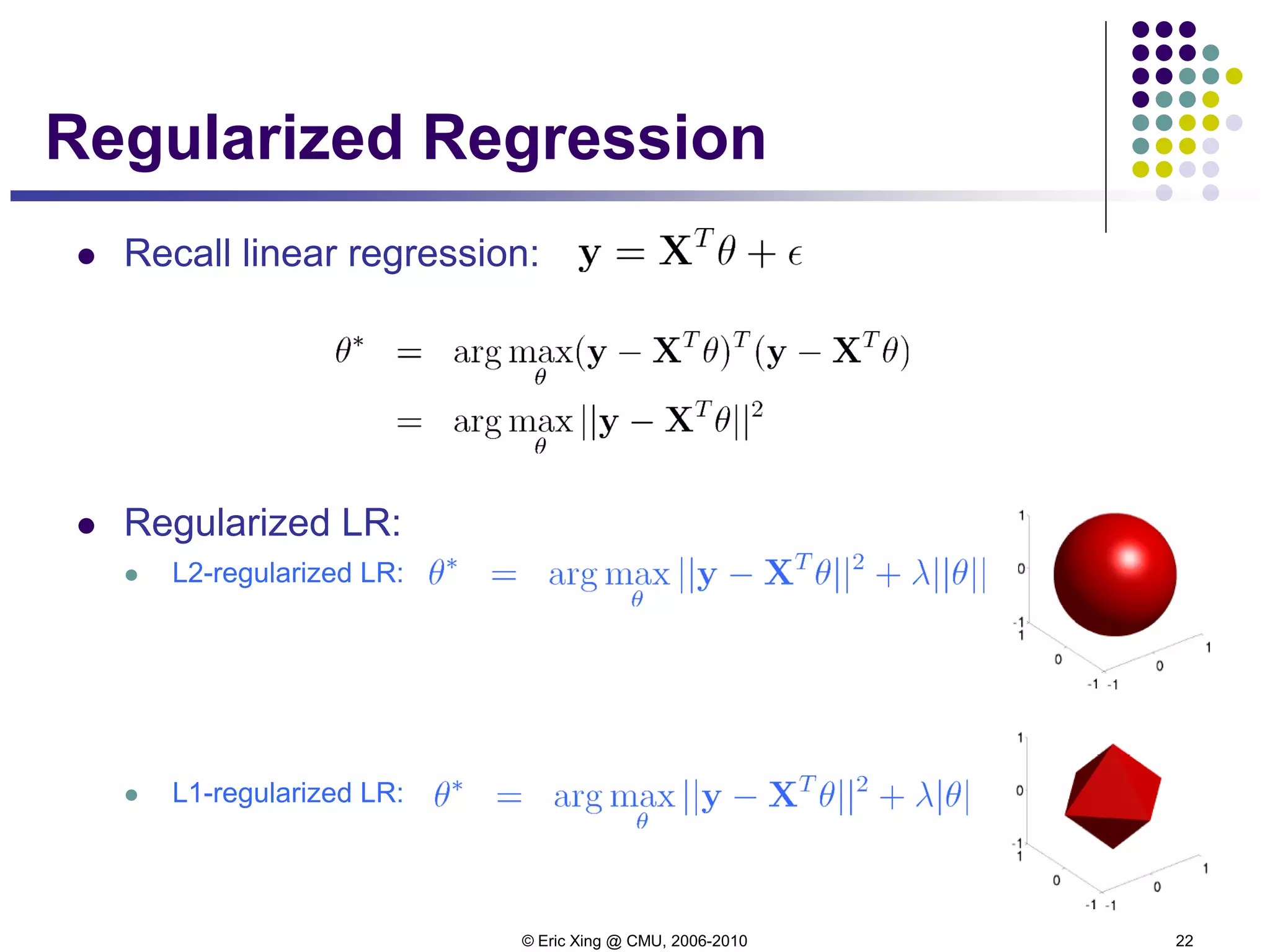
2. Regularization
 Maximum-likelihood estimates are not always the best (James
and Stein showed a counter example in the early 60's)
 Alternative: we "regularize" the likelihood objective (also
known as penalized likelihood, shrinkage, smoothing, etc.), by
adding to it a penalty term:
where λ>0 and ||θ|| might be the L1 or L2 norm.
 The choice of norm has an effect
 using the L2 norm pulls directly towards the origin,
 while using the L1 norm pulls towards the coordinate axes, i.e it tries to set some
of the coordinates to 0.
 This second approach can be useful in a feature-selection setting.
[ ]θλθθ
θ
+= );(maxargˆ
shrinkage Dl

30. © Eric Xing @ CMU, 2006-2010 31
Recall Bayesian and Frequentist
 Frequentist interpretation of probability
 Probabilities are objective properties of the real world, and refer to limiting relative
frequencies (e.g., number of times I have observed heads). Hence one cannot
write P(Katrina could have been prevented|D), since the event will never repeat.
 Parameters of models are fixed, unknown constants. Hence one cannot write
P(θ|D) since θ does not have a probability distribution. Instead one can only write
P(D|θ).
 One computes point estimates of parameters using various estimators, θ*= f(D),
which are designed to have various desirable qualities when averaged over future
data D (assumed to be drawn from the “true” distribution).
 Bayesian interpretation of probability
 Probability describes degrees of belief, not limiting frequencies.
 Parameters of models are hidden variables, so one can compute P(θ|D) or
P(f(θ)|D) for some function f.
 One estimates parameters by computing P(θ|D) using Bayes rule:
)(
)()|(
)(
Dp
pDp
Dθp
θθ
=

31. © Eric Xing @ CMU, 2006-2010 32
Bayesian interpretation of
regulation
 Regularized Linear Regression
 Recall that using squared error as the cost function results in the LMS estimate
 And assume iid data and Gaussian noise, LMS is equivalent to MLE of θ
 Now assume that vector θ follows a normal prior with 0-mean and a diagonal
covariance matrix
 What is the posterior distribution of θ?
∑=
−−=
n
i i
T
iynl 1
2
2
2
11
2
1
)(log)( xθ
σσπ
θ
),(~ IN 2
0 τθ
( ) ( ) { }2
1
2
2
22
2
2
1
2 τθ/(θCxθy
σ
πσθpD|θp
D,θpDθp
T
n
i
i
T
n
n/
−×






−−==
∝
∑=
−
expexp)()(
)()(

32. © Eric Xing @ CMU, 2006-2010 33
Bayesian interpretation of
regulation, con'd
 The posterior distribution of θ
 This leads to a now objective
 This is L2 regularized LR! --- a MAP estimation of θ
 What about L1 regularized LR! (homework)
 How to choose λ.
 cross-validation!
θλθ
θ
τ
θ
σ
θ
+=
−−−= ∑∑ ==
);(
2
11
)(
2
1
2
1
);( 1
2
21
2
2
Dl
yDl
K
k k
n
i i
T
iMAP x
( ) { }2
1
2
2
2
2
1
τθ/θxθy
σ
Dθp T
n
i
i
T
n −×






−−∝ ∑=
expexp)(

33. © Eric Xing @ CMU, 2006-2010 34
3. Feature Selection
 Imagine that you have a supervised learning problem where
the number of features d is very large (perhaps d
>>#samples), but you suspect that there is only a small
number of features that are "relevant" to the learning task.
 VC-theory can tell you that this scenario is likely to lead to
high generalization error – the learned model will potentially
overfit unless the training set is fairly large.
 So lets get rid of useless parameters!

34. © Eric Xing @ CMU, 2006-2010 35
How to score features
 How do you know which features can be pruned?
 Given labeled data, we can compute some simple score S(i) that
measures how informative each feature xi is about the class labels y.
 Ranking criteria:
 Mutual Information: score each feature by its mutual information with respect
to the class labels
 Bayes error:
 Redundancy (Markov-blank score) …
 We need estimate the relevant p()'s from data, e.g., using MLE
∑ ∑∈ ∈
=
},{ },{ )()(
),(
log),(),(
10 10ix y i
i
ii
ypxp
yxp
yxpyxMI

35. © Eric Xing @ CMU, 2006-2010 36
Feature Ranking
 Bayes error of each gene
 information gain for each
genes with respect to the
given partition
 KL of each removal gene
w.r.t. to its MB

36. © Eric Xing @ CMU, 2006-2010 37
Feature selection schemes
 Given n features, there are 2n possible feature subsets (why?)
 Thus feature selection can be posed as a model selection
problem over 2n possible models.
 For large values of n, it's usually too expensive to explicitly
enumerate over and compare all 2n models. Some heuristic
search procedure is used to find a good feature subset.
 Three general approaches:
 Filter: i.e., direct feature ranking, but taking no consideration of the subsequent
learning algorithm
 add (from empty set) or remove (from the full set) features one by one based on S(i)
 Cheap, but is subject to local optimality and may be unrobust under different classifiers
 Wrapper: determine the (inclusion or removal of) features based on performance
under the learning algorithms to be used. See next slide
 Simultaneous learning and feature selection.
 E.x. L1 regularized LR, Bayesian feature selection (will not cover in this class), etc.

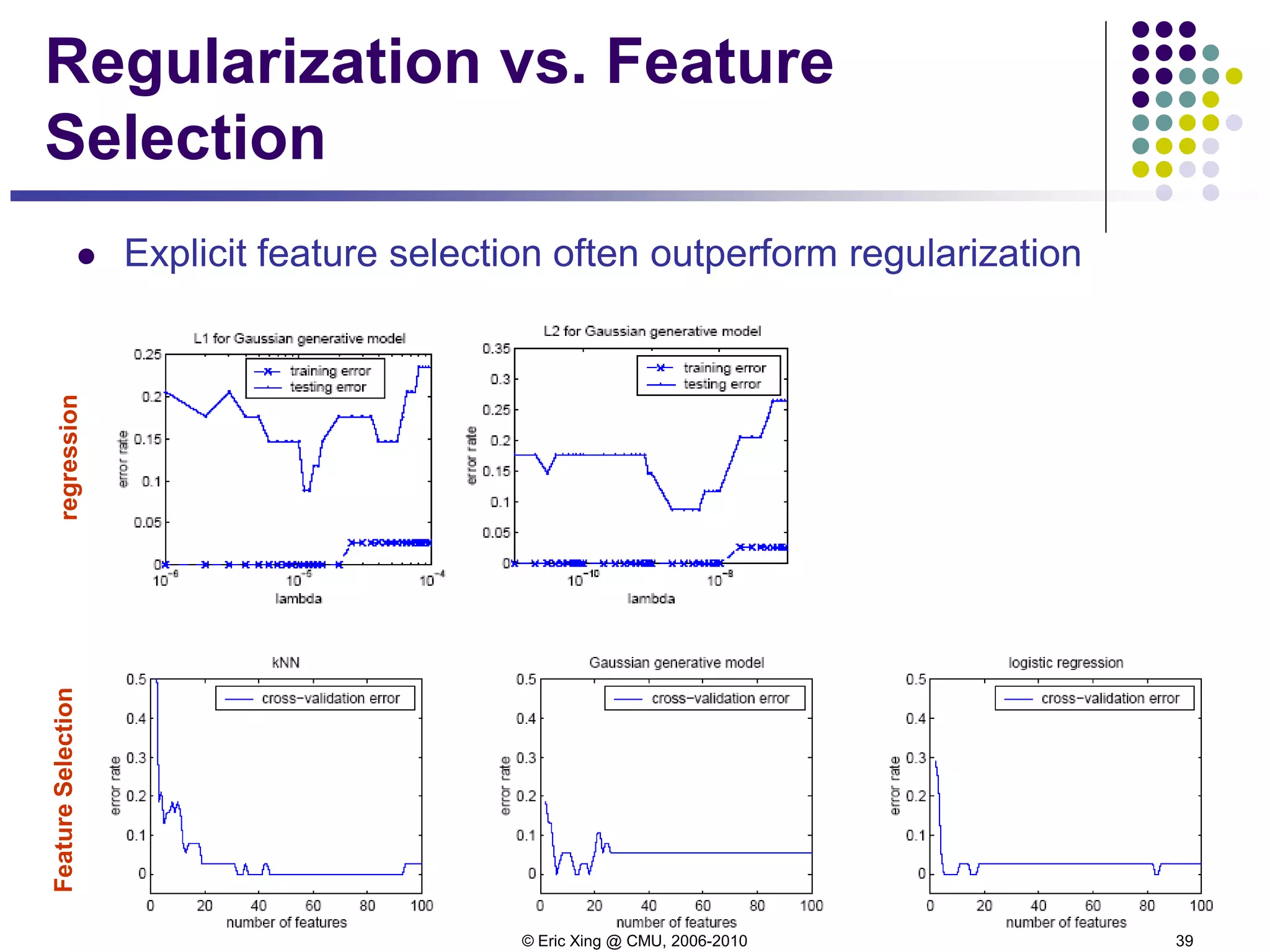
37. © Eric Xing @ CMU, 2006-2010 38
Case study [Xing et al, 2001]
 The case:
 7130 genes from a microarray dataset
 72 samples
 47 type I Leukemias (called ALL)
and 25 type II Leukemias (called AML)
 Three classifier:
 kNN
 Gaussian classifier
 Logistic regression

38. © Eric Xing @ CMU, 2006-2010 39
Regularization vs. Feature
Selection
 Explicit feature selection often outperform regularization
regressionFeatureSelection

39. © Eric Xing @ CMU, 2006-2010 40
4. Information criterion
 Suppose we are trying select among several different models
for a learning problem.
 The Problem:
 Given model family , find s.t.
 We can design J that not only reflect the predictive loss, but
also the amount of information Mk can hold
{ }IMMM ,,, 21=F F∈iM
),(maxarg MDJM
M
i
F∈
=

40. © Eric Xing @ CMU, 2006-2010 41
Model Selection via Information
Criteria
 Let f(x) denote the truth, the underlying distribution of the data
 Let g(x,θ) denote the model family we are evaluating
 f(x) does not necessarily reside in the model family
 θML(y) denote the MLE of model parameter from data y
 Among early attempts to move beyond Fisher's Maliximum
Likelihood framework, Akaike proposed the following
information criterion:
which is, of course, intractable (because f(x) is unknown)
( )[ ])(|( yxgfDE MLy θ

41. © Eric Xing @ CMU, 2006-2010 42
AIC and TIC
 AIC (An information criterion, not Akaike information criterion)
where k is the number of parameters in the model
 TIC (Takeuchi information criterion)
where
 We can approximate these terms in various ways (e.g., using the bootstrap)

kyxgA −= ))(ˆ|(log θ
))((tr))(ˆ|(log Σ−= 0θθ IyxgA
))|((minarg θθ ⋅= gfD0 ( )( )T
y yyE 00 θθθθ −−=Σ )(ˆ)(ˆ
0
2
0
θθ
θθ
θ
θ
=






∂∂
∂
−=
)|(log
)( Tx
xg
EI
kI ≈Σ))((tr 0θ

42. © Eric Xing @ CMU, 2006-2010 43
5. Bayesian Model Averaging
 Recall the Bayesian Theory: (e.g., for date D and model M)
P(M|D) = P(D|M)P(M)/P(D)
 the posterior equals to the likelihood times the prior, up to a constant.
 Assume that P(M) is uniform and notice that P(D) is constant,
we have the following criteria:
 A few steps of approximations (you will see this in advanced ML
class in later semesters) give you this:
where N is the number of data points in D.
∫=
θ
θθθ dMPMDPMDP )|(),|()|(
N
k
DPMDP ML log)ˆ|(log)|(
2
−≈ θ

43. © Eric Xing @ CMU, 2006-2010 44
Summary
 Structural risk minimization
 Bias-variance decomposition
 The battle against overfitting:
 Cross validation
 Regularization
 Feature selection
 Model selection --- Occam's razor
 Model averaging
 The Bayesian-frequentist debate
 Bayesian learning (weight models by their posterior probabilities)