SlideShare a Scribd company logo
Statistical learning theory was introduced in the late 1960s
but until 1990s it was simply a problem of function
estimation from a given collection of data.
In the middle of the 1990s, new types of learning algorithms
(e.g., support vector machines) based on the developed
theory were proposed.
This made statistical learning theory not only a tool for
theoretical analysis but also a tool for creating practical
algorithms for estimating multidimensional functions.
Statistical Learning and Model Selection
A good learner is the one which has good prediction accuracy; in other words, which has the
smallest prediction error.
• Statistical learning plays a key role in many areas of science,
finance, and industry. Some more examples of the learning
problems are:
• Predict whether a patient, hospitalized due to a heart attack,
will have a second heart attack. The prediction is to be based
on demographic, diet and clinical measurements for that
patient.
• Predict the price of a stock in 6 months from now, on the basis
of company performance measures and economic data.
• Estimate the amount of glucose in the blood of a diabetic
person, from the infrared absorption spectrum of that person’s
blood.
• Identify the risk factors for prostate cancer, based on clinical
and demographic variables.
• The science of learning plays a key role in the fields of
statistics, data mining, and artificial intelligence,
intersecting with areas of engineering and other
disciplines.
• The abstract learning theory of the 1960s established
more generalized conditions compared to those
discussed in classical statistical paradigms.
• Understanding these conditions inspired new
algorithmic approaches to function estimation problems.
• In essence, a statistical learning problem is learning from
the data. In a typical scenario, we have an outcome
measurement, usually quantitative (such as a stock price)
or categorical (such as heart attack/no heart attack), that
we wish to predict based on a set of features (such as
diet and clinical measurements).
• We have a Training Set which is used to observe the
outcome and feature measurements for a set of objects.
• Using this data we build a Prediction Model, or
a Statistical Learner, which enables us to predict the
outcome for a set of new unseen objects.
A good learner is one that accurately predicts such
an outcome.
• The examples considered above are all supervised
learning.
• All statistical learning problems may be constructed so
as to minimize expected loss.
• Mathematically, the problem of learning is that of
choosing from a given set of functions, the one that
predicts the supervised learning's response in the best
possible way.
• In order to choose the best available response, a risk
function is minimized in a situation where the joint
distribution of the predictors and response is unknown
and the only available information is obtained from the
training data.
The formulation of the learning problem is quite general.
However, two main types of problems are that of
• Regression Estimation
• Classification
• In the current course only these two are considered.
• The problem of regression estimation is the problem of
minimizing the risk functional with the squared error loss
function.
• When the problem is of classification, the loss function is an
indicator function.
• Hence, the problem is that of finding a function that
minimizes the misclassification error.
• There are several aspects of the model building process or
the process of finding an appropriate learning function.
• In what proportion data is allocated to certain tasks like
model building and evaluating model performance, is an
important aspect of modeling.
• How much data should be allocated to the training and test
sets? It generally depends on the situation.
• If the pool of data is small, the data splitting decisions can
be critical.
• Large data sets reduce the criticality of these
decisions.
• Before evaluating a model's predictive
performance in the test data, quantitative
assessments of the model using resampling
techniques helps to understand how
alternative models are expected to perform on
new data.
• Simple visualization, like a residual plot in case of
a regression, would also help.
• It is always a good practice to try out alternative
models.
• There is no single model that will always do better
than any other model for all datasets.
• Because of this, a strong case can be made to try
a wide variety of techniques, then determine
which model to focus on.
• Cross-validation, as well as the performance of a
model on the test data, help to make the final
decision.
• A model is a good fit, if it provides a high R2 value.
• However, note that the model has used all the observed
data and only the observed data.
• Hence, how it will perform when predicting for a new
set of input values (the predictor vector), is not clear.
• Assumption is that, with a high R2 value, the model is
expected to predict well for data observed in the
future.
• Suppose now the model is more complex than a linear model and a
spline smoother or a polynomial regression needs to be considered.
What would be the proper complexity of the model?
• Would it be a fifth-degree polynomial or a cubic spline would suffice?
Many modern classification and regression models are highly
adaptable and are capable of formulating complex relationships.
• At the same time they may overemphasize patterns that are not
reproducible.
• Without a methodological approach to evaluating models, the problem
will not be detected until the next set of samples are predicted.
• And here we are not talking about the data quality of the sample,
which is used to develop the model, being bad!
• The data at hand is to be used to find the best predictive
model. Almost all predictive modeling techniques have
tuning parameters that enable the model to flex to find the
structure in the data.
• Hence, we must use the existing data to identify settings for
the model’s parameters that yield the best and most realistic
predictive performance (known as model tuning) for future.
• Traditionally, this has been achieved by splitting the existing
data into training and test sets.
• The training set is used to build and tune the model and the
test set is used to estimate the model’s predictive
performance.
• Modern approaches to model building split the data into
multiple training and test sets, which have often been shown
to get more optimal tuning parameters and give a more
accurate representation of the model’s predictive
performance.
• More on data splitting is discussed in the next subsection.
• Let us consider the general regression problem. The training data,
• Dtraining = {(Xi, Yi), i = 1, 2, . . . , n}
• is used to regress Y on X, and then a new response, Ynew, is estimated
by applying the fiNtted model to a brand-new set of predictors, Xnew,
from the test set Dtest. Prediction for Ynew is done by multiplying the
new predictor values by the regression coefficients already obtained
from training set.
• The resulting prediction is compared with the actual response value.
Prediction Error
• The Prediction Error, PE, is defined as the mean squared error in predicting Ynew using f^(Xnew).
• PE = E[(Ynew − f^(Xnew))2], where the expectation is taken over (Xnew, Ynew). We
can estimate PE by:
The dilemma of developing a statistical learning algorithm is clear.
The model can be made very accurate based on the observed data.
However since the model is evaluated on its predictive ability on
unseen observations, there is no guarantee that the closest model to the
observed data will have the highest predictive accuracy for future data!
In fact, more often than not, it will NOT be.
Training and Test Error as A Function of Model Complexity
• Let us again go back to the multiple regression problem. Fit of a model improves with the
complexity of the model, i.e. as more predictors are included in the model the R2 value is
expected to improve. If predictors truly capture the main features behind the data, then they are
retained in the model. The trick to build an accurate predictive model is not to overfit the model to
the training data.
Overfitting a Model
• If a learning technique learns the structure of a training data too well then the model is applied to
the data on which the model was built, it correctly predicts every sample value. In the extreme
case the model in training data admits no error. In addition to learning the general patterns in the
data, the model has also learned the characteristics of each training data point's unique noise. This
type of model is said to be over-fit and will usually have poor accuracy when predicting a new
sample. (Why?)
Bias-Variance Trade-off
• Since this course deals with multiple linear regression and several other regression
methods, let us concentrate on the inherent problem of bias-variance trade off in
that context. However, the problem is completely general and is at the core of
coming up with a good predictive model.
• When the outcome is quantitative (as opposed to qualitative), the most common
method for characterizing a model’s predictive capabilities is to use the root mean
squared error (RMSE). This metric is a function of the model residuals, which are
the observed values minus the model predictions. The mean squared error (MSE) is
calculated by squaring the residuals and summing them. The value is usually
interpreted as either how far (on average) the residuals are from zero or as the
average distance between the observed values and the model predictions.
• If we assume that the data points are statistically independent and that the residuals
have a theoretical mean of zero and a constant variance σ2, then
E[MSE] = σ2 + (Model Bias)2 + Model Variance
The first term, σ2, is the irreducible error and cannot be eliminated by modeling.
The second term is the squared bias of themodel.
This reflects how close the functional form of the model is to the true relationship
between the predictors and the outcome.
If the true functional form in the population is parabolic and a linear model is
used, then the model is a biased model.
It is part of systematic error in the model.
The third part is the model variance.
It quantifies the dependency of a model on the data points, that are used to create
the model.
If change in a small portion of the data results in a substantial change in the
estimates of the model parameters, the model is said to have high variance.
The best learner is the one which can balance the bias and the variance of a
model.
• A biased model typically has low variance. An extreme example is when a
polynomial regression model is estimated by a constant value equal to the sample
median.
• The straight line will have no impact if a handful of observations are changed.
• However, bias of this model is excessively high and naturally it is not a good
model to consider.
• On the other extreme, suppose a model is constructed where the regression line is
made to go through all data points, or through as many of them as possible. This
model will have very high variance, as even if a single observed value is changed,
the model changes.
• Thus it is possible that when an intentional bias is introduced in a regression
model, the prediction error becomes smaller, compared to an unbiased regression
model.
• Ridge regression and Lasso are examples of that. While a simple
model has high bias, model complexity causes model variance to
increase.
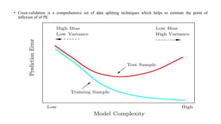
• An ideal predictor is that, which will learn all the structure in the data
but none of the noise. While with increasing model complexity in the
training data, PE reduces monotonically, the same will not be true for
test data.
• Bias and variance move in opposing directions and at a suitable bias-
variance combination the PE is the minimum in the test data.
• The model that achieves this lowest possible PE is the best prediction
model. The following figure is a graphical representation of that fact.
• Cross-validation is a comprehensive set of data splitting techniques which helps to estimate the point of
inflexion of of PE
• We mentioned that cross-validation is a technique to measure the
predictive performance of a model.
• Here we will explain the different methods of cross-validation (CV)
and their peculiarities.
Holdout Sample: Training and Test Data
• Data is split into two groups.
• The training set is used to train the learner.
• The test set is used to estimate the error rate of the trained
model. This method has two basic drawbacks.
• In a sparse data set, one may not have the luxury to set aside a
reasonable portion of the data for testing.
• Since it is a single repetition of the train-&-test experiment, the error
estimate is not stable. If we happen to have a 'bad' split, the estimate
is not reliable.
Three-way Split: Training, Validation and Test Data
• The available data is partitioned into three sets: training,
validation and test set. The prediction model is trained on the
training set and is evaluated on the validation set. For example,
in the case of a neural network, the training set is used to find the
optimal weights with the back-propagation rule. The validation set
may be used to find the optimum number of hidden layers or to
determine a stopping rule for the back-propagation
algorithm.Training and validation may be iterated a few times till a
'best' model is found. The final model is assessed using the test
set.
• A typical split is 50% for the training data and 25% each for
validation set and test set.
• With a three-way split, the model selection and the true error rate
computation can be carried out simultaneously. The error rate
estimate of the final model on validation data will be biased
(smaller than the true error rate) since the validation set is used to
select the final model. Hence a third independent part of the data,
the test data, is required.
• After assessing the final model on the test set, the model
must not be fine-tuned any further.
• Unfortunately, data insufficiency often does not allow three-
way split.
• The limitations of the holdout or three-way split can be overcome
with a family of resampling methods at the expense of higher
computational cost.
• Cross-Validation Among the methods available for estimating prediction
error, the most widely used is cross-validation (Stone, 1974).
• Essentially cross-validation includes techniques to split the sample into
multiple training and test data sets.
• Random Subsampling Random subsampling performs K data splits of the
entire sample.
• For each data split, a fixed number of observations is chosen without
replacement from the sample and kept aside as the test data.
• The prediction model is fitted to the training data from scratch for each of
the K splits and an estimate of prediction error is obtained from each test
set.
• Let the estimated PE in i-th test set be denoted by Ei .
• The true error estimate is obtained as the average of the separate
estimates Ei .
K-fold Cross-Validation
• A K-fold partition of the sample space is created.
• The original sample is randomly partitioned into K equal sized (or almost equal
sized) subsamples.
• Of the K subsamples, a single subsample is retained as the test set for
estimating the PE, and the remaining K-1 subsamples are used as training
data.
• The cross-validation process is then repeated K times (the folds), with each of
the K subsamples used exactly once as the test set.
• The K error estimates from the folds can then be averaged to produce a single
estimation.
• The advantage of this method is that all observations are used for both
training and validation, and each observation is used for validation exactly
once.
• For classification problems, one typically uses stratified K-fold cross-validation,
in which the folds are selected so that each fold contains roughly the same
proportions of class labels
• In repeated cross-validation, the cross-validation procedure is
repeated m times, yielding m random partitions of the original
sample.
• The m results are again averaged (or otherwise combined) to produce
a single estimation.
• A common choice for K is 10. With a large number of folds (K large)
the bias of the true error rate estimator is small but the variance will
be large.
• The computational time may also be very large as well, depending on
the complexity of the models under consideration.
• With a small number of folds the variance of the estimator will be small but
the bias will be large.
• The estimate may be larger than the true error rate. In practice the choice
of the number of folds depends on the size of the data set.
• For large data set, smaller K (e.g. 3) may yield quite accurate results. For
sparse data sets, Leave-one-out (LOO or LOOCV) may need to be used.
Leave-One-Out Cross-Validation
• LOO is the degenerate case of K-fold cross-validation where K = n for a
sample of size n.
• That means that n separate times, the prediction function is trained on all
the data except for one point and a prediction is made for that point.
• As before the average error is computed and used to evaluate the model.
• The evaluation given by leave-one-out cross validation error is good, but
sometimes it may be very expensive to compute

More Related Content

Similar to Statistical Learning and Model Selection module 2.pptx

datascience.docx
datascience.docxdatascience.docx
datascience.docx
JayaKulshrestha
 
Statistics for DP Biology IA
Statistics for DP Biology IAStatistics for DP Biology IA
Statistics for DP Biology IA
Veronika Garga
 
Top 10 Data Science Practitioner Pitfalls
Top 10 Data Science Practitioner PitfallsTop 10 Data Science Practitioner Pitfalls
Top 10 Data Science Practitioner Pitfalls
Sri Ambati
 
L7 method validation and modeling
L7 method validation and modelingL7 method validation and modeling
L7 method validation and modeling
Seppo Karrila
 
Sample and effect size
Sample and effect sizeSample and effect size
Sample and effect size
Sarithrakamalesan
 
Sample Size Calculations for Impact Evaluations
Sample Size Calculations for Impact EvaluationsSample Size Calculations for Impact Evaluations
Sample Size Calculations for Impact Evaluations
Marcos Vera
 
Pharmacokinetic pharmacodynamic modeling
Pharmacokinetic pharmacodynamic modelingPharmacokinetic pharmacodynamic modeling
Pharmacokinetic pharmacodynamic modeling
Meghana Gowda
 
Sample-size-comprehensive.pptx
Sample-size-comprehensive.pptxSample-size-comprehensive.pptx
Sample-size-comprehensive.pptx
ssuser4eb7dd
 
Machine learning - session 4
Machine learning - session 4Machine learning - session 4
Machine learning - session 4
Luis Borbon
 
4.1.pptx
4.1.pptx4.1.pptx
Test appraisal
Test appraisalTest appraisal
Test appraisal
AbdullahMir3
 
Dowhy: An end-to-end library for causal inference
Dowhy: An end-to-end library for causal inferenceDowhy: An end-to-end library for causal inference
Dowhy: An end-to-end library for causal inference
Amit Sharma
 
AI PROJECTppt.pptx
AI PROJECTppt.pptxAI PROJECTppt.pptx
AI PROJECTppt.pptx
ChocoMinati
 
cadd.pptx
cadd.pptxcadd.pptx
Systematic review and meta analysis
Systematic review and meta analysisSystematic review and meta analysis
Systematic review and meta analysis
umaisashraf
 
AI_Unit-4_Learning.pptx
AI_Unit-4_Learning.pptxAI_Unit-4_Learning.pptx
AI_Unit-4_Learning.pptx
MohammadAsim91
 
Regression analysis made easy
Regression analysis made easyRegression analysis made easy
Regression analysis made easy
Weam Banjar
 
Module 1 SLP 1I collected the data on the time.docx
Module 1 SLP 1I collected the data on the time.docxModule 1 SLP 1I collected the data on the time.docx
Module 1 SLP 1I collected the data on the time.docx
annandleola
 
LR 9 Estimation.pdf
LR 9 Estimation.pdfLR 9 Estimation.pdf
LR 9 Estimation.pdf
giovanniealvarez1
 

Similar to Statistical Learning and Model Selection module 2.pptx (20)

datascience.docx
datascience.docxdatascience.docx
datascience.docx
 
Statistics for DP Biology IA
Statistics for DP Biology IAStatistics for DP Biology IA
Statistics for DP Biology IA
 
Top 10 Data Science Practitioner Pitfalls
Top 10 Data Science Practitioner PitfallsTop 10 Data Science Practitioner Pitfalls
Top 10 Data Science Practitioner Pitfalls
 
L7 method validation and modeling
L7 method validation and modelingL7 method validation and modeling
L7 method validation and modeling
 
Sample and effect size
Sample and effect sizeSample and effect size
Sample and effect size
 
Sample Size Calculations for Impact Evaluations
Sample Size Calculations for Impact EvaluationsSample Size Calculations for Impact Evaluations
Sample Size Calculations for Impact Evaluations
 
Pharmacokinetic pharmacodynamic modeling
Pharmacokinetic pharmacodynamic modelingPharmacokinetic pharmacodynamic modeling
Pharmacokinetic pharmacodynamic modeling
 
Sample-size-comprehensive.pptx
Sample-size-comprehensive.pptxSample-size-comprehensive.pptx
Sample-size-comprehensive.pptx
 
Machine learning - session 4
Machine learning - session 4Machine learning - session 4
Machine learning - session 4
 
4.1.pptx
4.1.pptx4.1.pptx
4.1.pptx
 
Test appraisal
Test appraisalTest appraisal
Test appraisal
 
Unit 2 - Statistics
Unit 2 - StatisticsUnit 2 - Statistics
Unit 2 - Statistics
 
Dowhy: An end-to-end library for causal inference
Dowhy: An end-to-end library for causal inferenceDowhy: An end-to-end library for causal inference
Dowhy: An end-to-end library for causal inference
 
AI PROJECTppt.pptx
AI PROJECTppt.pptxAI PROJECTppt.pptx
AI PROJECTppt.pptx
 
cadd.pptx
cadd.pptxcadd.pptx
cadd.pptx
 
Systematic review and meta analysis
Systematic review and meta analysisSystematic review and meta analysis
Systematic review and meta analysis
 
AI_Unit-4_Learning.pptx
AI_Unit-4_Learning.pptxAI_Unit-4_Learning.pptx
AI_Unit-4_Learning.pptx
 
Regression analysis made easy
Regression analysis made easyRegression analysis made easy
Regression analysis made easy
 
Module 1 SLP 1I collected the data on the time.docx
Module 1 SLP 1I collected the data on the time.docxModule 1 SLP 1I collected the data on the time.docx
Module 1 SLP 1I collected the data on the time.docx
 
LR 9 Estimation.pdf
LR 9 Estimation.pdfLR 9 Estimation.pdf
LR 9 Estimation.pdf
 

More from nagarajan740445

principles of design thinking and start a new business in bengaluru.pptx
principles of design thinking and start a new business in bengaluru.pptxprinciples of design thinking and start a new business in bengaluru.pptx
principles of design thinking and start a new business in bengaluru.pptx
nagarajan740445
 
how to start the MSME business in India.pptx
how to start the MSME business in India.pptxhow to start the MSME business in India.pptx
how to start the MSME business in India.pptx
nagarajan740445
 
digital age mode Industry presentation.pptx
digital age mode Industry presentation.pptxdigital age mode Industry presentation.pptx
digital age mode Industry presentation.pptx
nagarajan740445
 
scorpio case study.pptx
scorpio case study.pptxscorpio case study.pptx
scorpio case study.pptx
nagarajan740445
 
SENCER_panel.ppt
SENCER_panel.pptSENCER_panel.ppt
SENCER_panel.ppt
nagarajan740445
 
geetha 1SP21BA009.pptx
geetha 1SP21BA009.pptxgeetha 1SP21BA009.pptx
geetha 1SP21BA009.pptx
nagarajan740445
 
gagana ppt 1.pptx
gagana ppt 1.pptxgagana ppt 1.pptx
gagana ppt 1.pptx
nagarajan740445
 
SCM + PUF_Day 3.pptx
SCM + PUF_Day 3.pptxSCM + PUF_Day 3.pptx
SCM + PUF_Day 3.pptx
nagarajan740445
 
Inroduction to ERP system core functions and challenages.pptx
Inroduction to ERP system core functions and challenages.pptxInroduction to ERP system core functions and challenages.pptx
Inroduction to ERP system core functions and challenages.pptx
nagarajan740445
 
MDD in CAP (Saundra Stock).ppt
MDD in CAP (Saundra Stock).pptMDD in CAP (Saundra Stock).ppt
MDD in CAP (Saundra Stock).ppt
nagarajan740445
 
Intestinal Obstruction (1).ppt
Intestinal Obstruction (1).pptIntestinal Obstruction (1).ppt
Intestinal Obstruction (1).ppt
nagarajan740445
 
marketing analytics 1.pptx
marketing analytics 1.pptxmarketing analytics 1.pptx
marketing analytics 1.pptx
nagarajan740445
 
first rule of marketing analytics forget about the customer.pptx
first rule of marketing analytics  forget about the customer.pptxfirst rule of marketing analytics  forget about the customer.pptx
first rule of marketing analytics forget about the customer.pptx
nagarajan740445
 
marketing analytics.pptx
marketing  analytics.pptxmarketing  analytics.pptx
marketing analytics.pptx
nagarajan740445
 
Cardiac.pptx
Cardiac.pptxCardiac.pptx
Cardiac.pptx
nagarajan740445
 
NERCOMPfinal_jfg.ppt
NERCOMPfinal_jfg.pptNERCOMPfinal_jfg.ppt
NERCOMPfinal_jfg.ppt
nagarajan740445
 
Data Analytics .pptx
Data Analytics .pptxData Analytics .pptx
Data Analytics .pptx
nagarajan740445
 
BUSINESS_ANALYTICS_ppt.ppt
BUSINESS_ANALYTICS_ppt.pptBUSINESS_ANALYTICS_ppt.ppt
BUSINESS_ANALYTICS_ppt.ppt
nagarajan740445
 
Tamil Nadul List of Doctors-2020.pdf
Tamil Nadul List of Doctors-2020.pdfTamil Nadul List of Doctors-2020.pdf
Tamil Nadul List of Doctors-2020.pdf
nagarajan740445
 
malabsorptionsyndrome-141120082515-conversion-gate02.pdf
malabsorptionsyndrome-141120082515-conversion-gate02.pdfmalabsorptionsyndrome-141120082515-conversion-gate02.pdf
malabsorptionsyndrome-141120082515-conversion-gate02.pdf
nagarajan740445
 

More from nagarajan740445 (20)

principles of design thinking and start a new business in bengaluru.pptx
principles of design thinking and start a new business in bengaluru.pptxprinciples of design thinking and start a new business in bengaluru.pptx
principles of design thinking and start a new business in bengaluru.pptx
 
how to start the MSME business in India.pptx
how to start the MSME business in India.pptxhow to start the MSME business in India.pptx
how to start the MSME business in India.pptx
 
digital age mode Industry presentation.pptx
digital age mode Industry presentation.pptxdigital age mode Industry presentation.pptx
digital age mode Industry presentation.pptx
 
scorpio case study.pptx
scorpio case study.pptxscorpio case study.pptx
scorpio case study.pptx
 
SENCER_panel.ppt
SENCER_panel.pptSENCER_panel.ppt
SENCER_panel.ppt
 
geetha 1SP21BA009.pptx
geetha 1SP21BA009.pptxgeetha 1SP21BA009.pptx
geetha 1SP21BA009.pptx
 
gagana ppt 1.pptx
gagana ppt 1.pptxgagana ppt 1.pptx
gagana ppt 1.pptx
 
SCM + PUF_Day 3.pptx
SCM + PUF_Day 3.pptxSCM + PUF_Day 3.pptx
SCM + PUF_Day 3.pptx
 
Inroduction to ERP system core functions and challenages.pptx
Inroduction to ERP system core functions and challenages.pptxInroduction to ERP system core functions and challenages.pptx
Inroduction to ERP system core functions and challenages.pptx
 
MDD in CAP (Saundra Stock).ppt
MDD in CAP (Saundra Stock).pptMDD in CAP (Saundra Stock).ppt
MDD in CAP (Saundra Stock).ppt
 
Intestinal Obstruction (1).ppt
Intestinal Obstruction (1).pptIntestinal Obstruction (1).ppt
Intestinal Obstruction (1).ppt
 
marketing analytics 1.pptx
marketing analytics 1.pptxmarketing analytics 1.pptx
marketing analytics 1.pptx
 
first rule of marketing analytics forget about the customer.pptx
first rule of marketing analytics  forget about the customer.pptxfirst rule of marketing analytics  forget about the customer.pptx
first rule of marketing analytics forget about the customer.pptx
 
marketing analytics.pptx
marketing  analytics.pptxmarketing  analytics.pptx
marketing analytics.pptx
 
Cardiac.pptx
Cardiac.pptxCardiac.pptx
Cardiac.pptx
 
NERCOMPfinal_jfg.ppt
NERCOMPfinal_jfg.pptNERCOMPfinal_jfg.ppt
NERCOMPfinal_jfg.ppt
 
Data Analytics .pptx
Data Analytics .pptxData Analytics .pptx
Data Analytics .pptx
 
BUSINESS_ANALYTICS_ppt.ppt
BUSINESS_ANALYTICS_ppt.pptBUSINESS_ANALYTICS_ppt.ppt
BUSINESS_ANALYTICS_ppt.ppt
 
Tamil Nadul List of Doctors-2020.pdf
Tamil Nadul List of Doctors-2020.pdfTamil Nadul List of Doctors-2020.pdf
Tamil Nadul List of Doctors-2020.pdf
 
malabsorptionsyndrome-141120082515-conversion-gate02.pdf
malabsorptionsyndrome-141120082515-conversion-gate02.pdfmalabsorptionsyndrome-141120082515-conversion-gate02.pdf
malabsorptionsyndrome-141120082515-conversion-gate02.pdf
 

Recently uploaded

Overview on Edible Vaccine: Pros & Cons with Mechanism
Overview on Edible Vaccine: Pros & Cons with MechanismOverview on Edible Vaccine: Pros & Cons with Mechanism
Overview on Edible Vaccine: Pros & Cons with Mechanism
DeeptiGupta154
 
Sha'Carri Richardson Presentation 202345
Sha'Carri Richardson Presentation 202345Sha'Carri Richardson Presentation 202345
Sha'Carri Richardson Presentation 202345
beazzy04
 
June 3, 2024 Anti-Semitism Letter Sent to MIT President Kornbluth and MIT Cor...
June 3, 2024 Anti-Semitism Letter Sent to MIT President Kornbluth and MIT Cor...June 3, 2024 Anti-Semitism Letter Sent to MIT President Kornbluth and MIT Cor...
June 3, 2024 Anti-Semitism Letter Sent to MIT President Kornbluth and MIT Cor...
Levi Shapiro
 
Polish students' mobility in the Czech Republic
Polish students' mobility in the Czech RepublicPolish students' mobility in the Czech Republic
Polish students' mobility in the Czech Republic
Anna Sz.
 
Welcome to TechSoup New Member Orientation and Q&A (May 2024).pdf
Welcome to TechSoup   New Member Orientation and Q&A (May 2024).pdfWelcome to TechSoup   New Member Orientation and Q&A (May 2024).pdf
Welcome to TechSoup New Member Orientation and Q&A (May 2024).pdf
TechSoup
 
678020731-Sumas-y-Restas-Para-Colorear.pdf
678020731-Sumas-y-Restas-Para-Colorear.pdf678020731-Sumas-y-Restas-Para-Colorear.pdf
678020731-Sumas-y-Restas-Para-Colorear.pdf
CarlosHernanMontoyab2
 
Mule 4.6 & Java 17 Upgrade | MuleSoft Mysore Meetup #46
Mule 4.6 & Java 17 Upgrade | MuleSoft Mysore Meetup #46Mule 4.6 & Java 17 Upgrade | MuleSoft Mysore Meetup #46
Mule 4.6 & Java 17 Upgrade | MuleSoft Mysore Meetup #46
MysoreMuleSoftMeetup
 
Additional Benefits for Employee Website.pdf
Additional Benefits for Employee Website.pdfAdditional Benefits for Employee Website.pdf
Additional Benefits for Employee Website.pdf
joachimlavalley1
 
A Strategic Approach: GenAI in Education
A Strategic Approach: GenAI in EducationA Strategic Approach: GenAI in Education
A Strategic Approach: GenAI in Education
Peter Windle
 
Honest Reviews of Tim Han LMA Course Program.pptx
Honest Reviews of Tim Han LMA Course Program.pptxHonest Reviews of Tim Han LMA Course Program.pptx
Honest Reviews of Tim Han LMA Course Program.pptx
timhan337
 
Model Attribute Check Company Auto Property
Model Attribute  Check Company Auto PropertyModel Attribute  Check Company Auto Property
Model Attribute Check Company Auto Property
Celine George
 
TESDA TM1 REVIEWER FOR NATIONAL ASSESSMENT WRITTEN AND ORAL QUESTIONS WITH A...
TESDA TM1 REVIEWER  FOR NATIONAL ASSESSMENT WRITTEN AND ORAL QUESTIONS WITH A...TESDA TM1 REVIEWER  FOR NATIONAL ASSESSMENT WRITTEN AND ORAL QUESTIONS WITH A...
TESDA TM1 REVIEWER FOR NATIONAL ASSESSMENT WRITTEN AND ORAL QUESTIONS WITH A...
EugeneSaldivar
 
The Roman Empire A Historical Colossus.pdf
The Roman Empire A Historical Colossus.pdfThe Roman Empire A Historical Colossus.pdf
The Roman Empire A Historical Colossus.pdf
kaushalkr1407
 
"Protectable subject matters, Protection in biotechnology, Protection of othe...
"Protectable subject matters, Protection in biotechnology, Protection of othe..."Protectable subject matters, Protection in biotechnology, Protection of othe...
"Protectable subject matters, Protection in biotechnology, Protection of othe...
SACHIN R KONDAGURI
 
The basics of sentences session 5pptx.pptx
The basics of sentences session 5pptx.pptxThe basics of sentences session 5pptx.pptx
The basics of sentences session 5pptx.pptx
heathfieldcps1
 
The Accursed House by Émile Gaboriau.pptx
The Accursed House by Émile Gaboriau.pptxThe Accursed House by Émile Gaboriau.pptx
The Accursed House by Émile Gaboriau.pptx
DhatriParmar
 
The geography of Taylor Swift - some ideas
The geography of Taylor Swift - some ideasThe geography of Taylor Swift - some ideas
The geography of Taylor Swift - some ideas
GeoBlogs
 
Operation Blue Star - Saka Neela Tara
Operation Blue Star   -  Saka Neela TaraOperation Blue Star   -  Saka Neela Tara
Operation Blue Star - Saka Neela Tara
Balvir Singh
 
How libraries can support authors with open access requirements for UKRI fund...
How libraries can support authors with open access requirements for UKRI fund...How libraries can support authors with open access requirements for UKRI fund...
How libraries can support authors with open access requirements for UKRI fund...
Jisc
 
BÀI TẬP BỔ TRỢ TIẾNG ANH GLOBAL SUCCESS LỚP 3 - CẢ NĂM (CÓ FILE NGHE VÀ ĐÁP Á...
BÀI TẬP BỔ TRỢ TIẾNG ANH GLOBAL SUCCESS LỚP 3 - CẢ NĂM (CÓ FILE NGHE VÀ ĐÁP Á...BÀI TẬP BỔ TRỢ TIẾNG ANH GLOBAL SUCCESS LỚP 3 - CẢ NĂM (CÓ FILE NGHE VÀ ĐÁP Á...
BÀI TẬP BỔ TRỢ TIẾNG ANH GLOBAL SUCCESS LỚP 3 - CẢ NĂM (CÓ FILE NGHE VÀ ĐÁP Á...
Nguyen Thanh Tu Collection
 

Recently uploaded (20)

Overview on Edible Vaccine: Pros & Cons with Mechanism
Overview on Edible Vaccine: Pros & Cons with MechanismOverview on Edible Vaccine: Pros & Cons with Mechanism
Overview on Edible Vaccine: Pros & Cons with Mechanism
 
Sha'Carri Richardson Presentation 202345
Sha'Carri Richardson Presentation 202345Sha'Carri Richardson Presentation 202345
Sha'Carri Richardson Presentation 202345
 
June 3, 2024 Anti-Semitism Letter Sent to MIT President Kornbluth and MIT Cor...
June 3, 2024 Anti-Semitism Letter Sent to MIT President Kornbluth and MIT Cor...June 3, 2024 Anti-Semitism Letter Sent to MIT President Kornbluth and MIT Cor...
June 3, 2024 Anti-Semitism Letter Sent to MIT President Kornbluth and MIT Cor...
 
Polish students' mobility in the Czech Republic
Polish students' mobility in the Czech RepublicPolish students' mobility in the Czech Republic
Polish students' mobility in the Czech Republic
 
Welcome to TechSoup New Member Orientation and Q&A (May 2024).pdf
Welcome to TechSoup   New Member Orientation and Q&A (May 2024).pdfWelcome to TechSoup   New Member Orientation and Q&A (May 2024).pdf
Welcome to TechSoup New Member Orientation and Q&A (May 2024).pdf
 
678020731-Sumas-y-Restas-Para-Colorear.pdf
678020731-Sumas-y-Restas-Para-Colorear.pdf678020731-Sumas-y-Restas-Para-Colorear.pdf
678020731-Sumas-y-Restas-Para-Colorear.pdf
 
Mule 4.6 & Java 17 Upgrade | MuleSoft Mysore Meetup #46
Mule 4.6 & Java 17 Upgrade | MuleSoft Mysore Meetup #46Mule 4.6 & Java 17 Upgrade | MuleSoft Mysore Meetup #46
Mule 4.6 & Java 17 Upgrade | MuleSoft Mysore Meetup #46
 
Additional Benefits for Employee Website.pdf
Additional Benefits for Employee Website.pdfAdditional Benefits for Employee Website.pdf
Additional Benefits for Employee Website.pdf
 
A Strategic Approach: GenAI in Education
A Strategic Approach: GenAI in EducationA Strategic Approach: GenAI in Education
A Strategic Approach: GenAI in Education
 
Honest Reviews of Tim Han LMA Course Program.pptx
Honest Reviews of Tim Han LMA Course Program.pptxHonest Reviews of Tim Han LMA Course Program.pptx
Honest Reviews of Tim Han LMA Course Program.pptx
 
Model Attribute Check Company Auto Property
Model Attribute  Check Company Auto PropertyModel Attribute  Check Company Auto Property
Model Attribute Check Company Auto Property
 
TESDA TM1 REVIEWER FOR NATIONAL ASSESSMENT WRITTEN AND ORAL QUESTIONS WITH A...
TESDA TM1 REVIEWER  FOR NATIONAL ASSESSMENT WRITTEN AND ORAL QUESTIONS WITH A...TESDA TM1 REVIEWER  FOR NATIONAL ASSESSMENT WRITTEN AND ORAL QUESTIONS WITH A...
TESDA TM1 REVIEWER FOR NATIONAL ASSESSMENT WRITTEN AND ORAL QUESTIONS WITH A...
 
The Roman Empire A Historical Colossus.pdf
The Roman Empire A Historical Colossus.pdfThe Roman Empire A Historical Colossus.pdf
The Roman Empire A Historical Colossus.pdf
 
"Protectable subject matters, Protection in biotechnology, Protection of othe...
"Protectable subject matters, Protection in biotechnology, Protection of othe..."Protectable subject matters, Protection in biotechnology, Protection of othe...
"Protectable subject matters, Protection in biotechnology, Protection of othe...
 
The basics of sentences session 5pptx.pptx
The basics of sentences session 5pptx.pptxThe basics of sentences session 5pptx.pptx
The basics of sentences session 5pptx.pptx
 
The Accursed House by Émile Gaboriau.pptx
The Accursed House by Émile Gaboriau.pptxThe Accursed House by Émile Gaboriau.pptx
The Accursed House by Émile Gaboriau.pptx
 
The geography of Taylor Swift - some ideas
The geography of Taylor Swift - some ideasThe geography of Taylor Swift - some ideas
The geography of Taylor Swift - some ideas
 
Operation Blue Star - Saka Neela Tara
Operation Blue Star   -  Saka Neela TaraOperation Blue Star   -  Saka Neela Tara
Operation Blue Star - Saka Neela Tara
 
How libraries can support authors with open access requirements for UKRI fund...
How libraries can support authors with open access requirements for UKRI fund...How libraries can support authors with open access requirements for UKRI fund...
How libraries can support authors with open access requirements for UKRI fund...
 
BÀI TẬP BỔ TRỢ TIẾNG ANH GLOBAL SUCCESS LỚP 3 - CẢ NĂM (CÓ FILE NGHE VÀ ĐÁP Á...
BÀI TẬP BỔ TRỢ TIẾNG ANH GLOBAL SUCCESS LỚP 3 - CẢ NĂM (CÓ FILE NGHE VÀ ĐÁP Á...BÀI TẬP BỔ TRỢ TIẾNG ANH GLOBAL SUCCESS LỚP 3 - CẢ NĂM (CÓ FILE NGHE VÀ ĐÁP Á...
BÀI TẬP BỔ TRỢ TIẾNG ANH GLOBAL SUCCESS LỚP 3 - CẢ NĂM (CÓ FILE NGHE VÀ ĐÁP Á...
 

Statistical Learning and Model Selection module 2.pptx

  • 1. Statistical learning theory was introduced in the late 1960s but until 1990s it was simply a problem of function estimation from a given collection of data. In the middle of the 1990s, new types of learning algorithms (e.g., support vector machines) based on the developed theory were proposed. This made statistical learning theory not only a tool for theoretical analysis but also a tool for creating practical algorithms for estimating multidimensional functions. Statistical Learning and Model Selection A good learner is the one which has good prediction accuracy; in other words, which has the smallest prediction error.
  • 2. • Statistical learning plays a key role in many areas of science, finance, and industry. Some more examples of the learning problems are: • Predict whether a patient, hospitalized due to a heart attack, will have a second heart attack. The prediction is to be based on demographic, diet and clinical measurements for that patient. • Predict the price of a stock in 6 months from now, on the basis of company performance measures and economic data. • Estimate the amount of glucose in the blood of a diabetic person, from the infrared absorption spectrum of that person’s blood. • Identify the risk factors for prostate cancer, based on clinical and demographic variables.
  • 3. • The science of learning plays a key role in the fields of statistics, data mining, and artificial intelligence, intersecting with areas of engineering and other disciplines. • The abstract learning theory of the 1960s established more generalized conditions compared to those discussed in classical statistical paradigms. • Understanding these conditions inspired new algorithmic approaches to function estimation problems.
  • 4. • In essence, a statistical learning problem is learning from the data. In a typical scenario, we have an outcome measurement, usually quantitative (such as a stock price) or categorical (such as heart attack/no heart attack), that we wish to predict based on a set of features (such as diet and clinical measurements). • We have a Training Set which is used to observe the outcome and feature measurements for a set of objects. • Using this data we build a Prediction Model, or a Statistical Learner, which enables us to predict the outcome for a set of new unseen objects.
  • 5. A good learner is one that accurately predicts such an outcome. • The examples considered above are all supervised learning. • All statistical learning problems may be constructed so as to minimize expected loss. • Mathematically, the problem of learning is that of choosing from a given set of functions, the one that predicts the supervised learning's response in the best possible way. • In order to choose the best available response, a risk function is minimized in a situation where the joint distribution of the predictors and response is unknown and the only available information is obtained from the training data.
  • 6. The formulation of the learning problem is quite general. However, two main types of problems are that of • Regression Estimation • Classification • In the current course only these two are considered. • The problem of regression estimation is the problem of minimizing the risk functional with the squared error loss function. • When the problem is of classification, the loss function is an indicator function. • Hence, the problem is that of finding a function that minimizes the misclassification error.
  • 7. • There are several aspects of the model building process or the process of finding an appropriate learning function. • In what proportion data is allocated to certain tasks like model building and evaluating model performance, is an important aspect of modeling. • How much data should be allocated to the training and test sets? It generally depends on the situation. • If the pool of data is small, the data splitting decisions can be critical.
  • 8. • Large data sets reduce the criticality of these decisions. • Before evaluating a model's predictive performance in the test data, quantitative assessments of the model using resampling techniques helps to understand how alternative models are expected to perform on new data. • Simple visualization, like a residual plot in case of a regression, would also help.
  • 9. • It is always a good practice to try out alternative models. • There is no single model that will always do better than any other model for all datasets. • Because of this, a strong case can be made to try a wide variety of techniques, then determine which model to focus on. • Cross-validation, as well as the performance of a model on the test data, help to make the final decision.
  • 10. • A model is a good fit, if it provides a high R2 value. • However, note that the model has used all the observed data and only the observed data. • Hence, how it will perform when predicting for a new set of input values (the predictor vector), is not clear. • Assumption is that, with a high R2 value, the model is expected to predict well for data observed in the future.
  • 11. • Suppose now the model is more complex than a linear model and a spline smoother or a polynomial regression needs to be considered. What would be the proper complexity of the model? • Would it be a fifth-degree polynomial or a cubic spline would suffice? Many modern classification and regression models are highly adaptable and are capable of formulating complex relationships. • At the same time they may overemphasize patterns that are not reproducible. • Without a methodological approach to evaluating models, the problem will not be detected until the next set of samples are predicted. • And here we are not talking about the data quality of the sample, which is used to develop the model, being bad!
  • 12. • The data at hand is to be used to find the best predictive model. Almost all predictive modeling techniques have tuning parameters that enable the model to flex to find the structure in the data. • Hence, we must use the existing data to identify settings for the model’s parameters that yield the best and most realistic predictive performance (known as model tuning) for future. • Traditionally, this has been achieved by splitting the existing data into training and test sets.
  • 13. • The training set is used to build and tune the model and the test set is used to estimate the model’s predictive performance. • Modern approaches to model building split the data into multiple training and test sets, which have often been shown to get more optimal tuning parameters and give a more accurate representation of the model’s predictive performance. • More on data splitting is discussed in the next subsection.
  • 14. • Let us consider the general regression problem. The training data, • Dtraining = {(Xi, Yi), i = 1, 2, . . . , n} • is used to regress Y on X, and then a new response, Ynew, is estimated by applying the fiNtted model to a brand-new set of predictors, Xnew, from the test set Dtest. Prediction for Ynew is done by multiplying the new predictor values by the regression coefficients already obtained from training set. • The resulting prediction is compared with the actual response value.
  • 15. Prediction Error • The Prediction Error, PE, is defined as the mean squared error in predicting Ynew using f^(Xnew). • PE = E[(Ynew − f^(Xnew))2], where the expectation is taken over (Xnew, Ynew). We can estimate PE by: The dilemma of developing a statistical learning algorithm is clear. The model can be made very accurate based on the observed data. However since the model is evaluated on its predictive ability on unseen observations, there is no guarantee that the closest model to the observed data will have the highest predictive accuracy for future data! In fact, more often than not, it will NOT be.
  • 16. Training and Test Error as A Function of Model Complexity • Let us again go back to the multiple regression problem. Fit of a model improves with the complexity of the model, i.e. as more predictors are included in the model the R2 value is expected to improve. If predictors truly capture the main features behind the data, then they are retained in the model. The trick to build an accurate predictive model is not to overfit the model to the training data. Overfitting a Model • If a learning technique learns the structure of a training data too well then the model is applied to the data on which the model was built, it correctly predicts every sample value. In the extreme case the model in training data admits no error. In addition to learning the general patterns in the data, the model has also learned the characteristics of each training data point's unique noise. This type of model is said to be over-fit and will usually have poor accuracy when predicting a new sample. (Why?)
  • 17. Bias-Variance Trade-off • Since this course deals with multiple linear regression and several other regression methods, let us concentrate on the inherent problem of bias-variance trade off in that context. However, the problem is completely general and is at the core of coming up with a good predictive model. • When the outcome is quantitative (as opposed to qualitative), the most common method for characterizing a model’s predictive capabilities is to use the root mean squared error (RMSE). This metric is a function of the model residuals, which are the observed values minus the model predictions. The mean squared error (MSE) is calculated by squaring the residuals and summing them. The value is usually interpreted as either how far (on average) the residuals are from zero or as the average distance between the observed values and the model predictions. • If we assume that the data points are statistically independent and that the residuals have a theoretical mean of zero and a constant variance σ2, then E[MSE] = σ2 + (Model Bias)2 + Model Variance
  • 18. The first term, σ2, is the irreducible error and cannot be eliminated by modeling. The second term is the squared bias of themodel. This reflects how close the functional form of the model is to the true relationship between the predictors and the outcome. If the true functional form in the population is parabolic and a linear model is used, then the model is a biased model. It is part of systematic error in the model. The third part is the model variance. It quantifies the dependency of a model on the data points, that are used to create the model. If change in a small portion of the data results in a substantial change in the estimates of the model parameters, the model is said to have high variance.
  • 19. The best learner is the one which can balance the bias and the variance of a model. • A biased model typically has low variance. An extreme example is when a polynomial regression model is estimated by a constant value equal to the sample median. • The straight line will have no impact if a handful of observations are changed. • However, bias of this model is excessively high and naturally it is not a good model to consider. • On the other extreme, suppose a model is constructed where the regression line is made to go through all data points, or through as many of them as possible. This model will have very high variance, as even if a single observed value is changed, the model changes. • Thus it is possible that when an intentional bias is introduced in a regression model, the prediction error becomes smaller, compared to an unbiased regression model.
  • 20. • Ridge regression and Lasso are examples of that. While a simple model has high bias, model complexity causes model variance to increase. • An ideal predictor is that, which will learn all the structure in the data but none of the noise. While with increasing model complexity in the training data, PE reduces monotonically, the same will not be true for test data. • Bias and variance move in opposing directions and at a suitable bias- variance combination the PE is the minimum in the test data. • The model that achieves this lowest possible PE is the best prediction model. The following figure is a graphical representation of that fact.
  • 21. • Cross-validation is a comprehensive set of data splitting techniques which helps to estimate the point of inflexion of of PE
  • 22. • We mentioned that cross-validation is a technique to measure the predictive performance of a model. • Here we will explain the different methods of cross-validation (CV) and their peculiarities. Holdout Sample: Training and Test Data • Data is split into two groups. • The training set is used to train the learner. • The test set is used to estimate the error rate of the trained model. This method has two basic drawbacks. • In a sparse data set, one may not have the luxury to set aside a reasonable portion of the data for testing. • Since it is a single repetition of the train-&-test experiment, the error estimate is not stable. If we happen to have a 'bad' split, the estimate is not reliable.
  • 23. Three-way Split: Training, Validation and Test Data • The available data is partitioned into three sets: training, validation and test set. The prediction model is trained on the training set and is evaluated on the validation set. For example, in the case of a neural network, the training set is used to find the optimal weights with the back-propagation rule. The validation set may be used to find the optimum number of hidden layers or to determine a stopping rule for the back-propagation algorithm.Training and validation may be iterated a few times till a 'best' model is found. The final model is assessed using the test set. • A typical split is 50% for the training data and 25% each for validation set and test set.
  • 24. • With a three-way split, the model selection and the true error rate computation can be carried out simultaneously. The error rate estimate of the final model on validation data will be biased (smaller than the true error rate) since the validation set is used to select the final model. Hence a third independent part of the data, the test data, is required. • After assessing the final model on the test set, the model must not be fine-tuned any further. • Unfortunately, data insufficiency often does not allow three- way split. • The limitations of the holdout or three-way split can be overcome with a family of resampling methods at the expense of higher computational cost.
  • 25. • Cross-Validation Among the methods available for estimating prediction error, the most widely used is cross-validation (Stone, 1974). • Essentially cross-validation includes techniques to split the sample into multiple training and test data sets. • Random Subsampling Random subsampling performs K data splits of the entire sample. • For each data split, a fixed number of observations is chosen without replacement from the sample and kept aside as the test data. • The prediction model is fitted to the training data from scratch for each of the K splits and an estimate of prediction error is obtained from each test set. • Let the estimated PE in i-th test set be denoted by Ei . • The true error estimate is obtained as the average of the separate estimates Ei .
  • 26. K-fold Cross-Validation • A K-fold partition of the sample space is created. • The original sample is randomly partitioned into K equal sized (or almost equal sized) subsamples. • Of the K subsamples, a single subsample is retained as the test set for estimating the PE, and the remaining K-1 subsamples are used as training data. • The cross-validation process is then repeated K times (the folds), with each of the K subsamples used exactly once as the test set. • The K error estimates from the folds can then be averaged to produce a single estimation. • The advantage of this method is that all observations are used for both training and validation, and each observation is used for validation exactly once. • For classification problems, one typically uses stratified K-fold cross-validation, in which the folds are selected so that each fold contains roughly the same proportions of class labels
  • 27. • In repeated cross-validation, the cross-validation procedure is repeated m times, yielding m random partitions of the original sample. • The m results are again averaged (or otherwise combined) to produce a single estimation. • A common choice for K is 10. With a large number of folds (K large) the bias of the true error rate estimator is small but the variance will be large. • The computational time may also be very large as well, depending on the complexity of the models under consideration.
  • 28. • With a small number of folds the variance of the estimator will be small but the bias will be large. • The estimate may be larger than the true error rate. In practice the choice of the number of folds depends on the size of the data set. • For large data set, smaller K (e.g. 3) may yield quite accurate results. For sparse data sets, Leave-one-out (LOO or LOOCV) may need to be used. Leave-One-Out Cross-Validation • LOO is the degenerate case of K-fold cross-validation where K = n for a sample of size n. • That means that n separate times, the prediction function is trained on all the data except for one point and a prediction is made for that point. • As before the average error is computed and used to evaluate the model. • The evaluation given by leave-one-out cross validation error is good, but sometimes it may be very expensive to compute