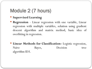
Module 2 (7hours)
Supervised Learning
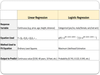
Regression - Linear regression with one variable, Linear
regression with multiple variables, solution using gradient
descent algorithm and matrix method, basic idea of
overfitting in regression.
Linear Methods for Classification- Logistic regression,
Naive Bayes, Decision tree
algorithm ID3.
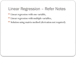
Linear Regression –Refer Notes
Linear regression with one variable,
Linear regression with multiple variables,
Solution using matrix method (derivation not required)
5.
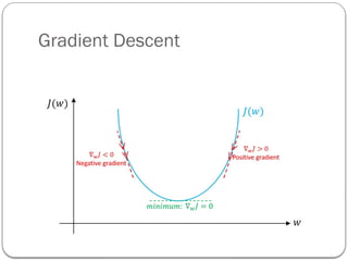
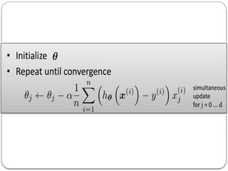
Gradient Descent Algorithm
Gradient Descent is the most common optimization
algorithm in machine learning and deep learning.
It is a first-order optimization algorithm.
This means it only takes into account the first derivative
when performing the updates on the parameters.
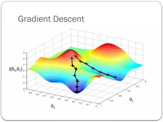
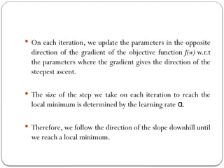
On eachiteration, we update the parameters in the opposite
direction of the gradient of the objective function J(w) w.r.t
the parameters where the gradient gives the direction of the
steepest ascent.
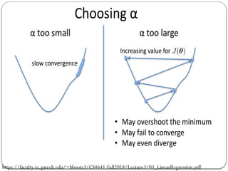
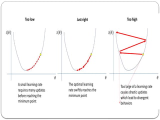
The size of the step we take on each iteration to reach the
local minimum is determined by the learning rate .
α
Therefore, we follow the direction of the slope downhill until
we reach a local minimum.
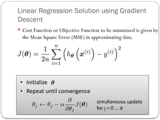
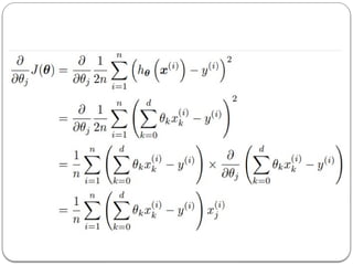
Linear Regression Solutionusing Gradient
Descent
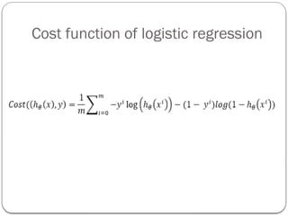
Cost Function or Objective Function to be minimized is given by
the Mean Square Error (MSE) in approximating data.
12.
Stochastic gradient descentalgorithm
On-line gradient descent, also known as sequential
gradient descent or stochastic gradient descent, makes an
update to the weight vector based on one data point at a
time.
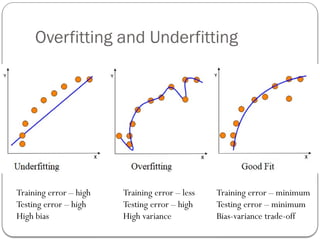
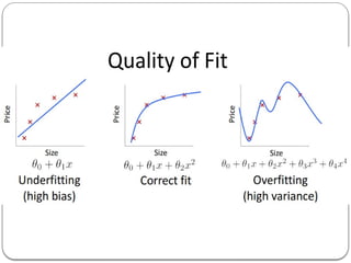
Overfitting and Underfitting
Trainingerror – less
Testing error – high
High variance
Training error – high
Testing error – high
High bias
Training error – minimum
Testing error – minimum
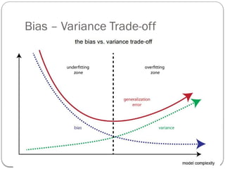
Bias-variance trade-off
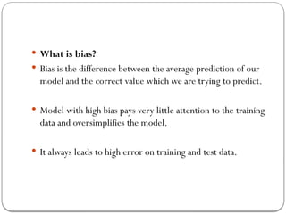
What isbias?
Bias is the difference between the average prediction of our
model and the correct value which we are trying to predict.
Model with high bias pays very little attention to the training
data and oversimplifies the model.
It always leads to high error on training and test data.
19.
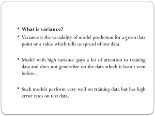
What isvariance?
Variance is the variability of model prediction for a given data
point or a value which tells us spread of our data.
Model with high variance pays a lot of attention to training
data and does not generalize on the data which it hasn’t seen
before.
Such models perform very well on training data but has high
error rates on test data.
20.
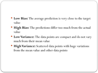
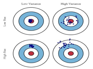
Low Bias:The average prediction is very close to the target
value
High Bias: The predictions differ too much from the actual
value
LowVariance: The data points are compact and do not vary
much from their mean value
HighVariance: Scattered data points with huge variations
from the mean value and other data points
22.
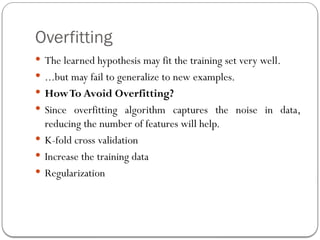
Overfitting
The learnedhypothesis may fit the training set very well.
...but may fail to generalize to new examples.
HowTo Avoid Overfitting?
Since overfitting algorithm captures the noise in data,
reducing the number of features will help.
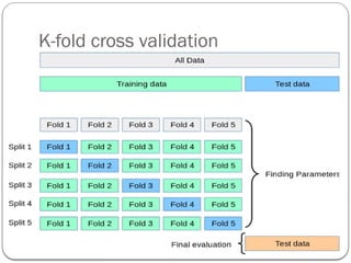
K-fold cross validation
Increase the training data
Regularization
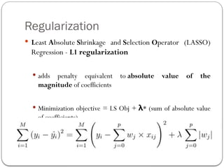
Regularization
Least AbsoluteShrinkage and Selection Operator (LASSO)
Regression - L1 regularization
adds penalty equivalent to absolute value of the
magnitude of coefficients
Minimization objective = LS Obj + λ* (sum of absolute value
of coefficients)
25.
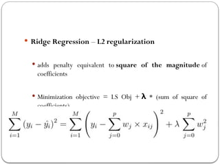
Ridge Regression– L2 regularization
adds penalty equivalent to square of the magnitude of
coefficients
Minimization objective = LS Obj + λ * (sum of square of
coefficients)
26.
HowTo AvoidUnderfitting?
Increasing the model complexity. e.g. If linear function under
fit then try using polynomial features
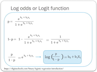
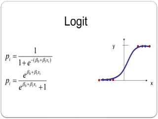
Log odds
Odds(odds of success): It is defined as the chances of
success divided by the chances of failure.
Odds = p/(1-p)
Log odds: It is the logarithm of the odds ratio.
Log odds = log[p/(1-p)]
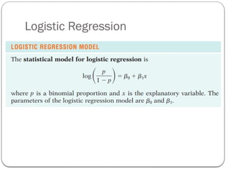
32.
Log odds orLogit function
https://digitaschools.com/binary-logistic-regression-introduction/
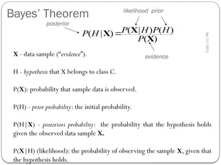
Bayes’ Theorem
06/21/2025
39
( |) ( )
( | )
( )
P H P H
P H
P
X
X
X
X - data sample (“evidence”).
H - hypothesis that X belongs to class C.
P(X): probability that sample data is observed.
P(H) - prior probability: the initial probability.
P(H|X) - posteriori probability: the probability that the hypothesis holds
given the observed data sample X.
P(X|H) (likelihood): the probability of observing the sample X, given that
the hypothesis holds.
posterior
likelihood prior
evidence
40.
40
Bayesian Classification: Why?
A statistical classifier: performs probabilistic prediction, i.e., predicts class
membership probabilities.
Foundation: Based on Bayes’Theorem.
Incremental: Each training example can incrementally increase/decrease
the probability that a hypothesis is correct — prior knowledge can be
combined with observed data.
06/21/2025
41.
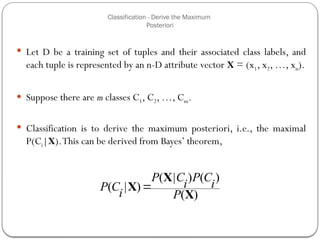
Classification - Derivethe Maximum
Posteriori
Let D be a training set of tuples and their associated class labels, and
each tuple is represented by an n-D attribute vector X = (x1, x2, …, xn).
Suppose there are m classes C1, C2, …, Cm.
Classification is to derive the maximum posteriori, i.e., the maximal
P(Ci|X).This can be derived from Bayes’ theorem,
)
(
)
(
)
|
(
)
|
(
X
X
X
P
i
C
P
i
C
P
i
C
P
41
42.
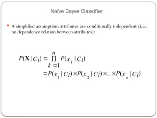
Naïve Bayes Classifier
A simplified assumption: attributes are conditionally independent (i.e.,
no dependence relation between attributes):
1 2
( | ) ( | )
1
( | ) ( | ) ... ( | )
k
n
n
P P
C x C
i i
k
P P P
x C x C x C
i i i
X
42
43.
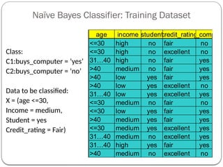
Naïve Bayes Classifier:Training Dataset
06/21/2025
43
age income student
credit_rating
buys_compute
<=30 high no fair no
<=30 high no excellent no
31…40 high no fair yes
>40 medium no fair yes
>40 low yes fair yes
>40 low yes excellent no
31…40 low yes excellent yes
<=30 medium no fair no
<=30 low yes fair yes
>40 medium yes fair yes
<=30 medium yes excellent yes
31…40 medium no excellent yes
31…40 high yes fair yes
>40 medium no excellent no
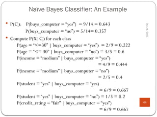
Class:
C1:buys_computer = ‘yes’
C2:buys_computer = ‘no’
Data to be classified:
X = (age <=30,
Income = medium,
Student = yes
Credit_rating = Fair)
06/21/2025
45
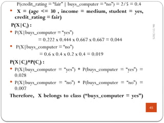
P(credit_rating = “fair”| buys_computer = “no”) = 2/5 = 0.4
X = (age <= 30 , income = medium, student = yes,
credit_rating = fair)
P(X|Ci) :
P(X|buys_computer = “yes”)
= 0.222 x 0.444 x 0.667 x 0.667 = 0.044
P(X|buys_computer = “no”)
= 0.6 x 0.4 x 0.2 x 0.4 = 0.019
P(X|Ci)*P(Ci) :
P(X|buys_computer = “yes”) * P(buys_computer = “yes”) =
0.028
P(X|buys_computer = “no”) * P(buys_computer = “no”) =
0.007
Therefore, X belongs to class (“buys_computer = yes”)
46.
06/21/2025
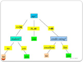
Decision Tree Induction– ID3
(Iterative Dichotomiser)
(by ROSS QUINLAN, 1986)
46
https://link.springer.com/content/pdf/10.1007/BF00116251.pdf
47.
06/21/2025
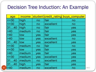
Decision Tree Induction:An Example
47
age income student credit_rating buys_computer
<=30 high no fair no
<=30 high no excellent no
31…40 high no fair yes
>40 medium no fair yes
>40 low yes fair yes
>40 low yes excellent no
31…40 low yes excellent yes
<=30 medium no fair no
<=30 low yes fair yes
>40 medium yes fair yes
<=30 medium yes excellent yes
31…40 medium no excellent yes
31…40 high yes fair yes
>40 medium no excellent no
Algorithm for DecisionTree Induction
06/21/2025
49
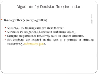
Basic algorithm (a greedy algorithm)
At start, all the training examples are at the root.
Attributes are categorical (discretize if continuous-valued).
Examples are partitioned recursively based on selected attributes.
Test attributes are selected on the basis of a heuristic or statistical
measure (e.g., information gain).
50.
06/21/2025
50
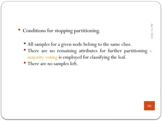
Conditions forstopping partitioning.
All samples for a given node belong to the same class.
There are no remaining attributes for further partitioning –
majority voting is employed for classifying the leaf.
There are no samples left.
51.
06/21/2025
Attribute Selection Measures– Information
Gain
51
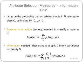
Let pi be the probability that an arbitrary tuple in D belongs to
class Ci, estimated by |Ci, D|/|D|.
Expected information (entropy) needed to classify a tuple in
D:
Information needed (after using A to split D into v partitions)
to classify D:
)
(
log
)
( 2
1
i
m
i
i p
p
D
Info
)
(
|
|
|
|
)
(
1
j
v
j
j
A D
Info
D
D
D
Info
52.
06/21/2025
52
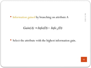
Information gainedby branching on attribute A
Select the attribute with the highest information gain.
(D)
Info
Info(D)
Gain(A) A
53.
06/21/2025
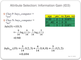
Attribute Selection: InformationGain (ID3)
53
g Class P: buys_computer =
“yes”
g Class N: buys_computer =
“no”
age yes no I(yes, no)
<=30 2 3 0.971
31…40 4 0 0
>40 3 2 0.971
5 4 5
( ) (2,3) (4,0) (3,2)
14 14 14
0.694
age
Info D I I I
2 2
( ) (9,5)
9 9 5 5
log ( ) log ( )
14 14 14 14
0.940
Info D I
54.
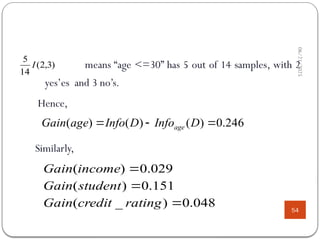
06/21/2025
54
means “age <=30”has 5 out of 14 samples, with 2
yes’es and 3 no’s.
Hence,
Similarly,
246
.
0
)
(
)
(
)
(
D
Info
D
Info
age
Gain age
)
3
,
2
(
14
5
I
048
.
0
)
_
(
151
.
0
)
(
029
.
0
)
(
rating
credit
Gain
student
Gain
income
Gain
Overfitting and TreePruning
06/21/2025
57
Overfitting: A decision tree may overfit the training data.
Two approaches to avoid overfitting:
Prepruning
Postpruning
Editor's Notes
#51 I : the expected information needed to classify a given sample
E (entropy) : expected information based on the partitioning into subsets by A

![Log odds
Odds (odds of success): It is defined as the chances of
success divided by the chances of failure.
Odds = p/(1-p)
Log odds: It is the logarithm of the odds ratio.
Log odds = log[p/(1-p)]](https://image.slidesharecdn.com/cst413ktus7csemachinelearningsupervisedlearningclassificationalgorithmsnaivebayesdecisiontreeslogist-250621082935-cc5685f8/85/CST413-KTU-S7-CSE-Machine-Learning-Supervised-Learning-Classification-Algorithms-Naive-Bayes-Decision-Trees-Logistic-Regression-Module-2-pptx-31-320.jpg)