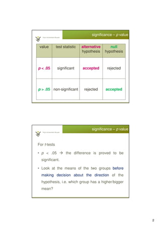
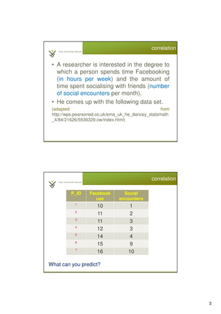
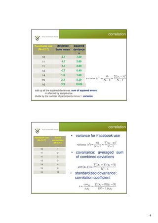
1
Introduction to applied statistics
& applied statistical methods
Prof. Dr. Chang Zhu1
objectives
• significance p-value
• Paired sample t-test
• Mann Whitney tests
• correlation
Pearson’s r
Spearman’s rho (rs)
Kendall’s tau-b (τ)
Partial correlation
2
significance – p value
value test statistic alternative
hypothesis
null
hypothesis
p < .05 significant accepted rejected
p > .05 non-significant rejected accepted
significance – p value
For t-tests
• p < .05 the difference is proved to be
significant.
• Look at the means of the two groups before
making decision about the direction of the
hypothesis, i.e. which group has a higher/bigger
mean?
3
correlation
• A researcher is interested in the degree to
which a person spends time Facebooking
(in hours per week) and the amount of
time spent socialising with friends (number
of social encounters per month).
• He comes up with the following data set.
(adapted from
http://wps.pearsoned.co.uk/ema_uk_he_dancey_statsmath
_4/84/21626/5536329.cw/index.html)
P_ID Facebook
use
Social
encounters
1
10 1
2
11 2
3
11 3
4
12 3
5
14 4
6
15 9
7
16 10
correlation
What can you predict?
4
Facebook use
(M=12.7)
deviance
from mean
squared
deviance
s
10 -2.7 7.29
11 -1.7 2.89
11 -1.7 2.89
12 -0.7 0.49
14 1.3 1.69
15 2.3 5.29
16 3.3 10.89
correlation
add up all the squared deviances: sum of squared errors
affected by sample size
divide by the number of participants minus 1: variance
Facebook use
(M=12.7)
Social
encounters
(M=6.14)
10 1
11 2
11 3
12 3
14 4
15 9
16 10
correlation
• variance for Facebook use
• covariance: averaged sum
of combined deviations
• standardized covariance:
correlation coefficient
5
correlation
SPSS output
Correlations
FB Encounters
FB
Pearson Correlation 1 .900**
Sig. (2-tailed) .006
N
7 7
Encounters
Pearson Correlation .900** 1
Sig. (2-tailed) .006
N 7 7
**. Correlation is significant at the 0.01 level (2-tailed).
r = .90, p < .01 (significant)
Correlation
Positive Correlation Negative Correlation
Correlation analysis
6
correlation
The correlation coefficient: measures the relative
strength of the linear relationship between two
variables
• Ranges between –1 and 1
• The closer to –1, the stronger the negative
linear relationship
• The closer to 1, the stronger the positive
linear relationship
• The closer to 0, the weaker any positive linear
relationship
A perfect positive correlation
Height
Weight
Height
of A
Weight
of A
Height
of B
Weight
of B
A linear
relationship
7
High Degree of positive correlation
• Positive relationship
Height
Weight
r = +.80
• Moderate Positive Correlation
Weight
Shoe
Size
r = + 0.4
8
• Perfect Negative Correlation
Exam score
TV
watching
per
week
r = -1.0
• Moderate Negative Correlation
Exam score
TV
watching
per
week
r = -.80
9
• Weak negative Correlation
Weight
Shoe
Size r = - 0.2
• No Correlation (horizontal line)
Height
IQ
r = 0.0
10
Test of Correlations
Parametric test:
Pearson’s r is the most common correlation coefficient.
Non-parametric tests
• Spearman’s rho (rs): rank the scores, then use the
same equation as above.
• Kendall’s tau-b (τ) : taking into account tied ranks.
PRACTICE
11
Practice 1
Pearson’s correlation
•We collect the scores of 200 high school students on
various tests, including science, reading, and maths score,
and we want to know if there is a correlation between the
scores of each pair of the variables.
•The data file is named test_score.sav
In SPSS, choose Analyse > Correlate > Bivariate
practical guidelines page 2
SPSS output
Correlations
reading score math score science score
reading score Pearson Correlation
1 .662** .630**
Sig. (2-tailed)
.000 .000
N 200 200 200
math score Pearson Correlation
.662** 1 .631**
Sig. (2-tailed)
.000 .000
N 200 200 200
science score Pearson Correlation
.630** .631** 1
Sig. (2-tailed)
.000 .000
N 200 200 200
**. Correlation is significant at the 0.01 level (2-tailed).
12
Practice 1
Conclusion?
Reading scores were significantly correlated with math
scores, r = .66, p < .01 (one-tailed), and science scores, r =
.63, p < .01 (one-tailed); the math scores were also correlated
with the science scores, r = .63, p < .01 (one-tailed).
(Practical guidelines page 4)
Practice 2
Partial correlation
• Use the data file Exam Anxiety.sav
• Conduct the Pearson’s correlation for the three variables:
exam, anxiety, and revise
• What is the relationship between the variable anxiety
and exam and revise
In SPSS, choose Analyse > Correlate > Bivariate
13
SPSS output
Correlations
Time Spent
Revising
Exam
Performance (%) Exam Anxiety
Time Spent
Revising
Pearson
Correlation 1 .397** -.709**
Sig. (2-tailed)
.000 .000
N 103 103 103
Exam
Performance (%)
Pearson
Correlation .397** 1 -.441**
Sig. (2-tailed)
.000 .000
N 103 103 103
Exam Anxiety Pearson
Correlation -.709** -.441** 1
Sig. (2-tailed)
.000 .000
N 103 103 103
**. Correlation is significant at the 0.01 level (2-tailed).
Practice 2
Partial correlation
Observation:
• Exam anxiety is negatively correlated with
exam performance (r = -.441)
• Exam anxiety is also negatively correlated
with the time spent revising (revision time)
for the exam (r = -.709)
• However, exam performance is positively
related to the time spent revising (r= .397)
14
Practice 2
Partial correlation
• The revision time may affect the relationship between
exam anxiety and exam performance such that the more
one spends time on revision, the less anxiety one
perceives, hence better performance.
• We are capable of investigating purely the relationship
between exam anxiety and exam performance, taking
into account the effect of time spent on revising.
In SPSS, choose Analyse > Correlate > Partial
SPSS output
Correlations
Control Variables Exam Performance (%) Exam Anxiety
Time Spent Revising
Exam Performance
(%)
Correlation
1.000 -.247
Significance (2-
tailed) . .012
df 0 100
Exam Anxiety Correlation -.247 1.000
Significance (2-
tailed) .012 .
df 100 0
not controlling for time spent revising: r = -.441
15
Practice 2
Partial correlation
Conclusion?
Exam anxiety was significantly related to exam performance,
r = -.247, p < .05 (two-tailed), controlling for the effect of time
spent on revising.
(Practical guidelines page 4)
Practice 1
•Two examiners rated the presentations of 20 students with 1
being poor and 10 meaning perfect. It is expected that the scores
would be similar.
•The data file is named presentation_rating.sav.
(Practical guidelines page 6)
Practice 3
Spearman and Kendall’s tau
(nonparametric)
In SPSS, choose Analyse > Correlate > Bivariate
16
Practice 3
Spearman and Kendall’s tau
(nonparametric)
Conclusion?
•The rating of the two examiners was significantly correlated, rs =
.825, p < .01 (one-tailed). Or:
•The rating of the two examiners was significantly correlated, τ =
.707, p < .01 (one-tailed)
(Practical guidelines page 6)
Assignment
• Conduct paired t-test
• Conduct Mann Whitney tests
• Conduct correlation analysis

Applied statistics lecture_4

  • 1.
    1 Introduction to appliedstatistics & applied statistical methods Prof. Dr. Chang Zhu1 objectives • significance p-value • Paired sample t-test • Mann Whitney tests • correlation Pearson’s r Spearman’s rho (rs) Kendall’s tau-b (τ) Partial correlation
  • 2.
    2 significance – pvalue value test statistic alternative hypothesis null hypothesis p < .05 significant accepted rejected p > .05 non-significant rejected accepted significance – p value For t-tests • p < .05 the difference is proved to be significant. • Look at the means of the two groups before making decision about the direction of the hypothesis, i.e. which group has a higher/bigger mean?
  • 3.
    3 correlation • A researcheris interested in the degree to which a person spends time Facebooking (in hours per week) and the amount of time spent socialising with friends (number of social encounters per month). • He comes up with the following data set. (adapted from http://wps.pearsoned.co.uk/ema_uk_he_dancey_statsmath _4/84/21626/5536329.cw/index.html) P_ID Facebook use Social encounters 1 10 1 2 11 2 3 11 3 4 12 3 5 14 4 6 15 9 7 16 10 correlation What can you predict?
  • 4.
    4 Facebook use (M=12.7) deviance from mean squared deviance s 10-2.7 7.29 11 -1.7 2.89 11 -1.7 2.89 12 -0.7 0.49 14 1.3 1.69 15 2.3 5.29 16 3.3 10.89 correlation add up all the squared deviances: sum of squared errors affected by sample size divide by the number of participants minus 1: variance Facebook use (M=12.7) Social encounters (M=6.14) 10 1 11 2 11 3 12 3 14 4 15 9 16 10 correlation • variance for Facebook use • covariance: averaged sum of combined deviations • standardized covariance: correlation coefficient
  • 5.
    5 correlation SPSS output Correlations FB Encounters FB PearsonCorrelation 1 .900** Sig. (2-tailed) .006 N 7 7 Encounters Pearson Correlation .900** 1 Sig. (2-tailed) .006 N 7 7 **. Correlation is significant at the 0.01 level (2-tailed). r = .90, p < .01 (significant) Correlation Positive Correlation Negative Correlation Correlation analysis
  • 6.
    6 correlation The correlation coefficient:measures the relative strength of the linear relationship between two variables • Ranges between –1 and 1 • The closer to –1, the stronger the negative linear relationship • The closer to 1, the stronger the positive linear relationship • The closer to 0, the weaker any positive linear relationship A perfect positive correlation Height Weight Height of A Weight of A Height of B Weight of B A linear relationship
  • 7.
    7 High Degree ofpositive correlation • Positive relationship Height Weight r = +.80 • Moderate Positive Correlation Weight Shoe Size r = + 0.4
  • 8.
    8 • Perfect NegativeCorrelation Exam score TV watching per week r = -1.0 • Moderate Negative Correlation Exam score TV watching per week r = -.80
  • 9.
    9 • Weak negativeCorrelation Weight Shoe Size r = - 0.2 • No Correlation (horizontal line) Height IQ r = 0.0
  • 10.
    10 Test of Correlations Parametrictest: Pearson’s r is the most common correlation coefficient. Non-parametric tests • Spearman’s rho (rs): rank the scores, then use the same equation as above. • Kendall’s tau-b (τ) : taking into account tied ranks. PRACTICE
  • 11.
    11 Practice 1 Pearson’s correlation •Wecollect the scores of 200 high school students on various tests, including science, reading, and maths score, and we want to know if there is a correlation between the scores of each pair of the variables. •The data file is named test_score.sav In SPSS, choose Analyse > Correlate > Bivariate practical guidelines page 2 SPSS output Correlations reading score math score science score reading score Pearson Correlation 1 .662** .630** Sig. (2-tailed) .000 .000 N 200 200 200 math score Pearson Correlation .662** 1 .631** Sig. (2-tailed) .000 .000 N 200 200 200 science score Pearson Correlation .630** .631** 1 Sig. (2-tailed) .000 .000 N 200 200 200 **. Correlation is significant at the 0.01 level (2-tailed).
  • 12.
    12 Practice 1 Conclusion? Reading scoreswere significantly correlated with math scores, r = .66, p < .01 (one-tailed), and science scores, r = .63, p < .01 (one-tailed); the math scores were also correlated with the science scores, r = .63, p < .01 (one-tailed). (Practical guidelines page 4) Practice 2 Partial correlation • Use the data file Exam Anxiety.sav • Conduct the Pearson’s correlation for the three variables: exam, anxiety, and revise • What is the relationship between the variable anxiety and exam and revise In SPSS, choose Analyse > Correlate > Bivariate
  • 13.
    13 SPSS output Correlations Time Spent Revising Exam Performance(%) Exam Anxiety Time Spent Revising Pearson Correlation 1 .397** -.709** Sig. (2-tailed) .000 .000 N 103 103 103 Exam Performance (%) Pearson Correlation .397** 1 -.441** Sig. (2-tailed) .000 .000 N 103 103 103 Exam Anxiety Pearson Correlation -.709** -.441** 1 Sig. (2-tailed) .000 .000 N 103 103 103 **. Correlation is significant at the 0.01 level (2-tailed). Practice 2 Partial correlation Observation: • Exam anxiety is negatively correlated with exam performance (r = -.441) • Exam anxiety is also negatively correlated with the time spent revising (revision time) for the exam (r = -.709) • However, exam performance is positively related to the time spent revising (r= .397)
  • 14.
    14 Practice 2 Partial correlation •The revision time may affect the relationship between exam anxiety and exam performance such that the more one spends time on revision, the less anxiety one perceives, hence better performance. • We are capable of investigating purely the relationship between exam anxiety and exam performance, taking into account the effect of time spent on revising. In SPSS, choose Analyse > Correlate > Partial SPSS output Correlations Control Variables Exam Performance (%) Exam Anxiety Time Spent Revising Exam Performance (%) Correlation 1.000 -.247 Significance (2- tailed) . .012 df 0 100 Exam Anxiety Correlation -.247 1.000 Significance (2- tailed) .012 . df 100 0 not controlling for time spent revising: r = -.441
  • 15.
    15 Practice 2 Partial correlation Conclusion? Examanxiety was significantly related to exam performance, r = -.247, p < .05 (two-tailed), controlling for the effect of time spent on revising. (Practical guidelines page 4) Practice 1 •Two examiners rated the presentations of 20 students with 1 being poor and 10 meaning perfect. It is expected that the scores would be similar. •The data file is named presentation_rating.sav. (Practical guidelines page 6) Practice 3 Spearman and Kendall’s tau (nonparametric) In SPSS, choose Analyse > Correlate > Bivariate
  • 16.
    16 Practice 3 Spearman andKendall’s tau (nonparametric) Conclusion? •The rating of the two examiners was significantly correlated, rs = .825, p < .01 (one-tailed). Or: •The rating of the two examiners was significantly correlated, τ = .707, p < .01 (one-tailed) (Practical guidelines page 6) Assignment • Conduct paired t-test • Conduct Mann Whitney tests • Conduct correlation analysis