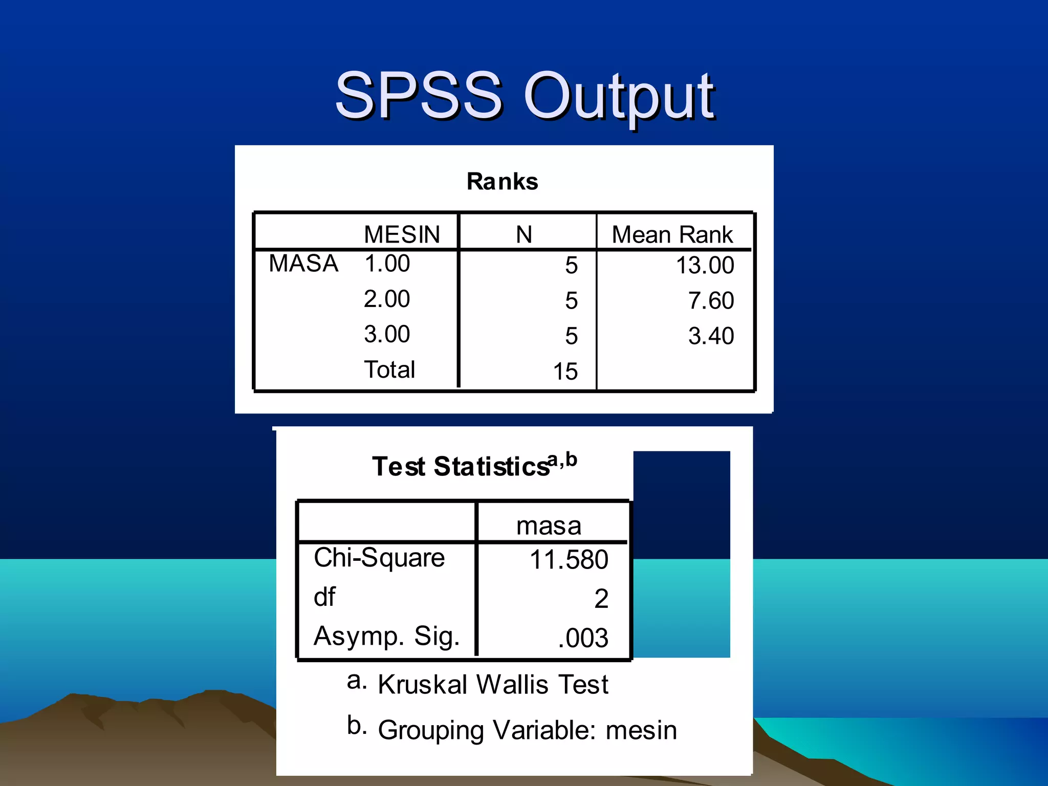
![SPSS Output
Ranks
KERJA N Mean Rank Sum of Ranks
GLU 1.00 3 5.00 15.00
3.00 5 4.20 21.00
Total 8
Test Statisticsb
GLU
Mann-Whitney U 6.000
Wilcoxon W 21.000
Z -.447
Asymp. Sig. (2-tailed) .655
Exact Sig. [2*(1-tailed a
.786
Sig.)]
a. Not corrected for ties.
b. Grouping Variable: KERJA](https://image.slidesharecdn.com/wilcoxonkruskal-120919030740-phpapp02/75/Non-parametric-analysis-Wilcoxon-Kruskal-Wallis-Spearman-16-2048.jpg)


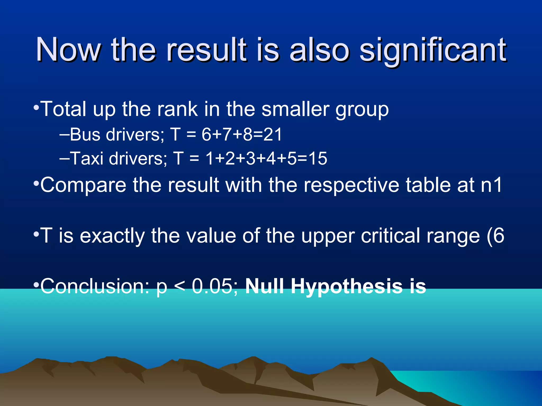

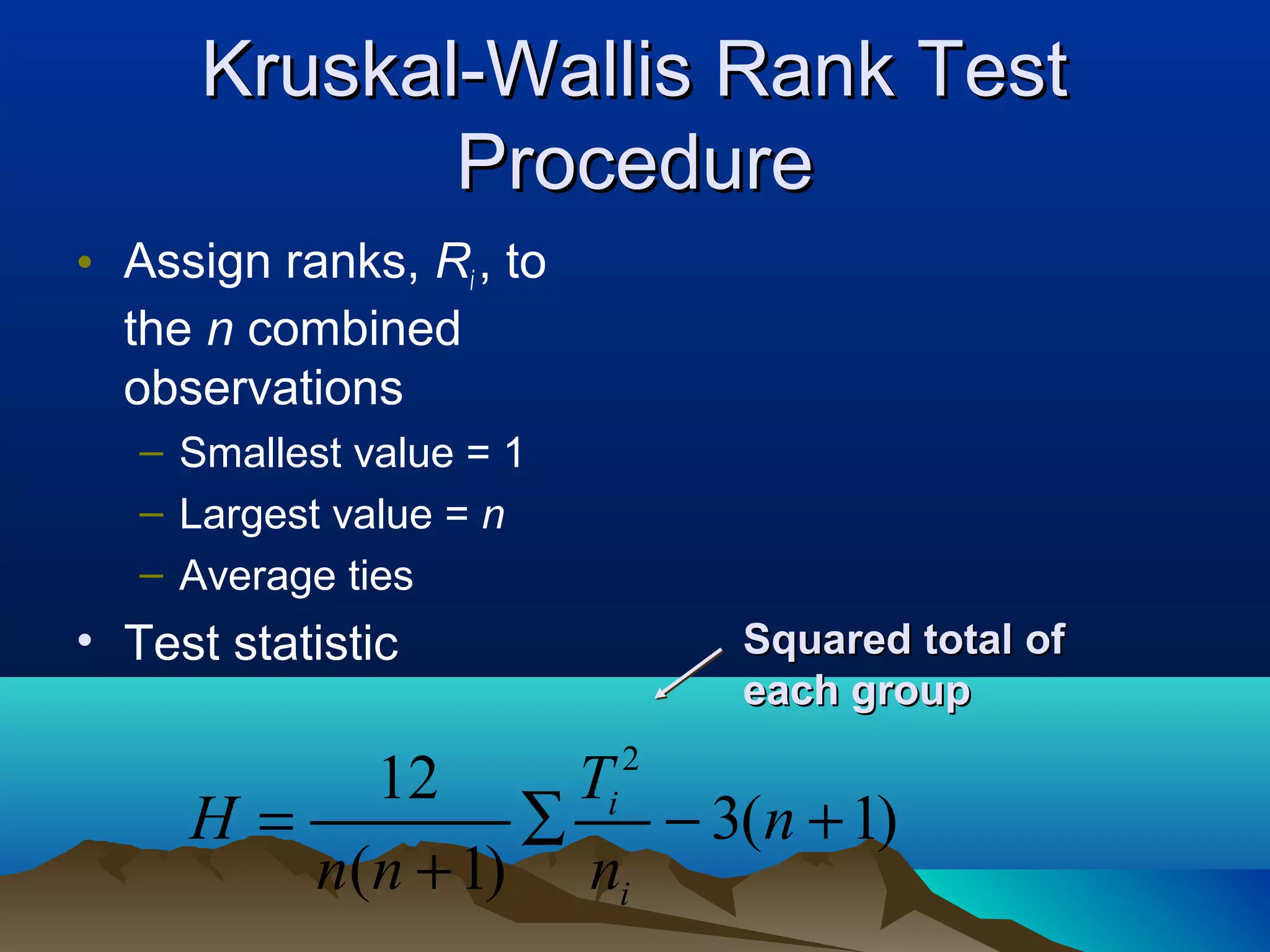
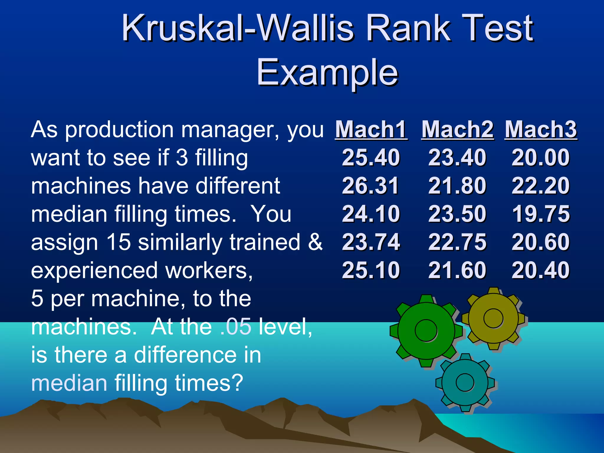
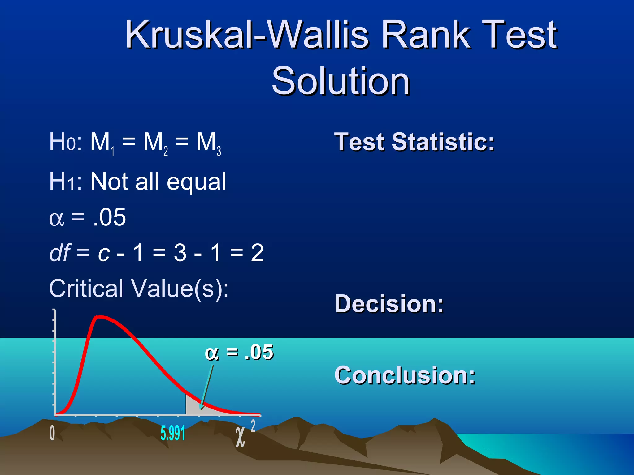
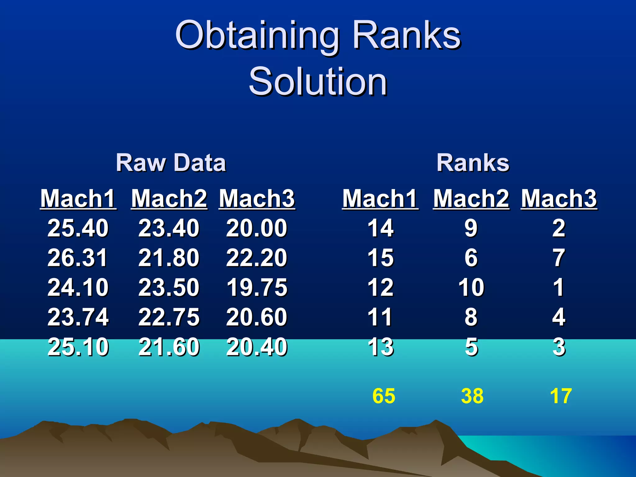

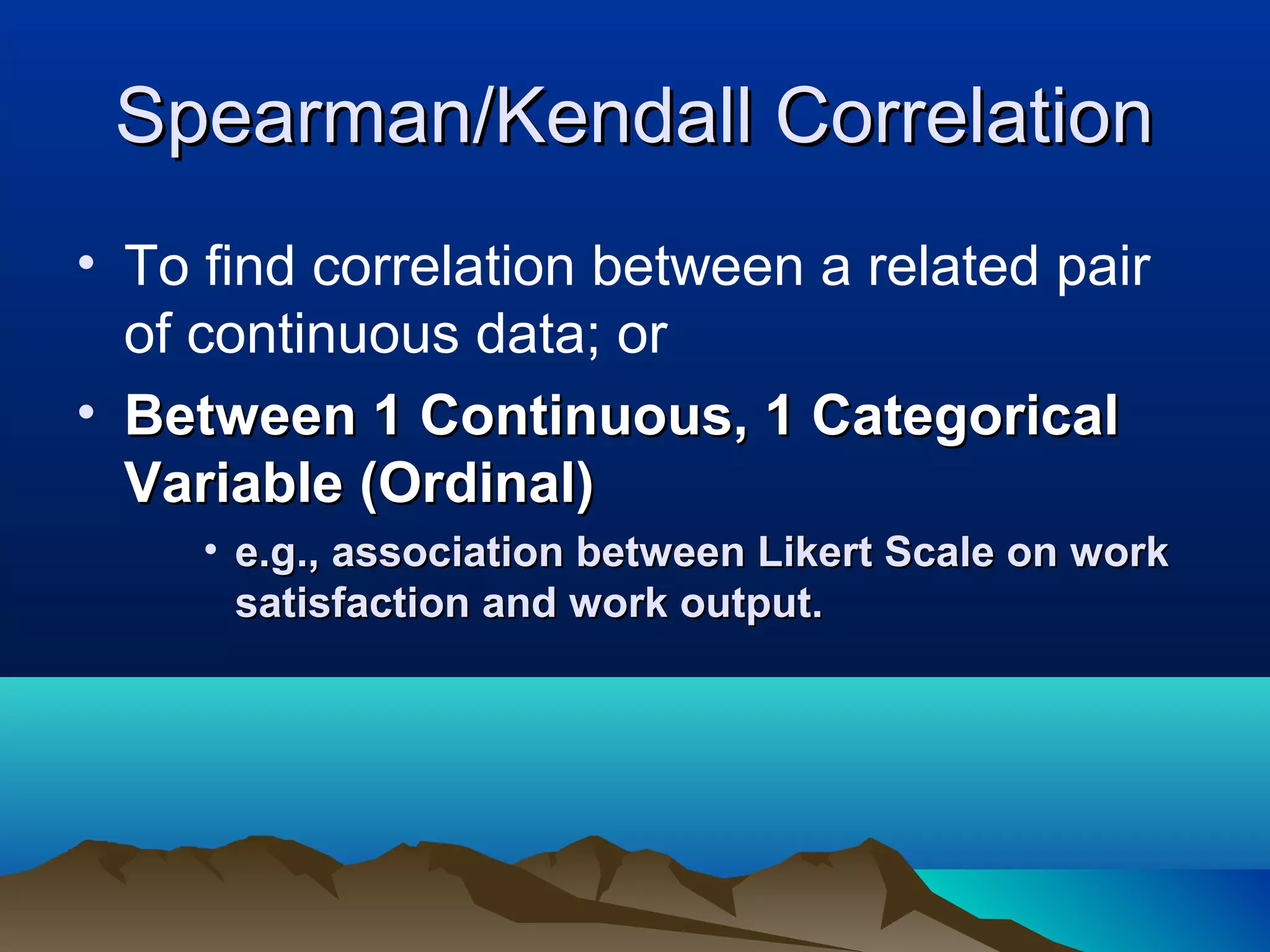
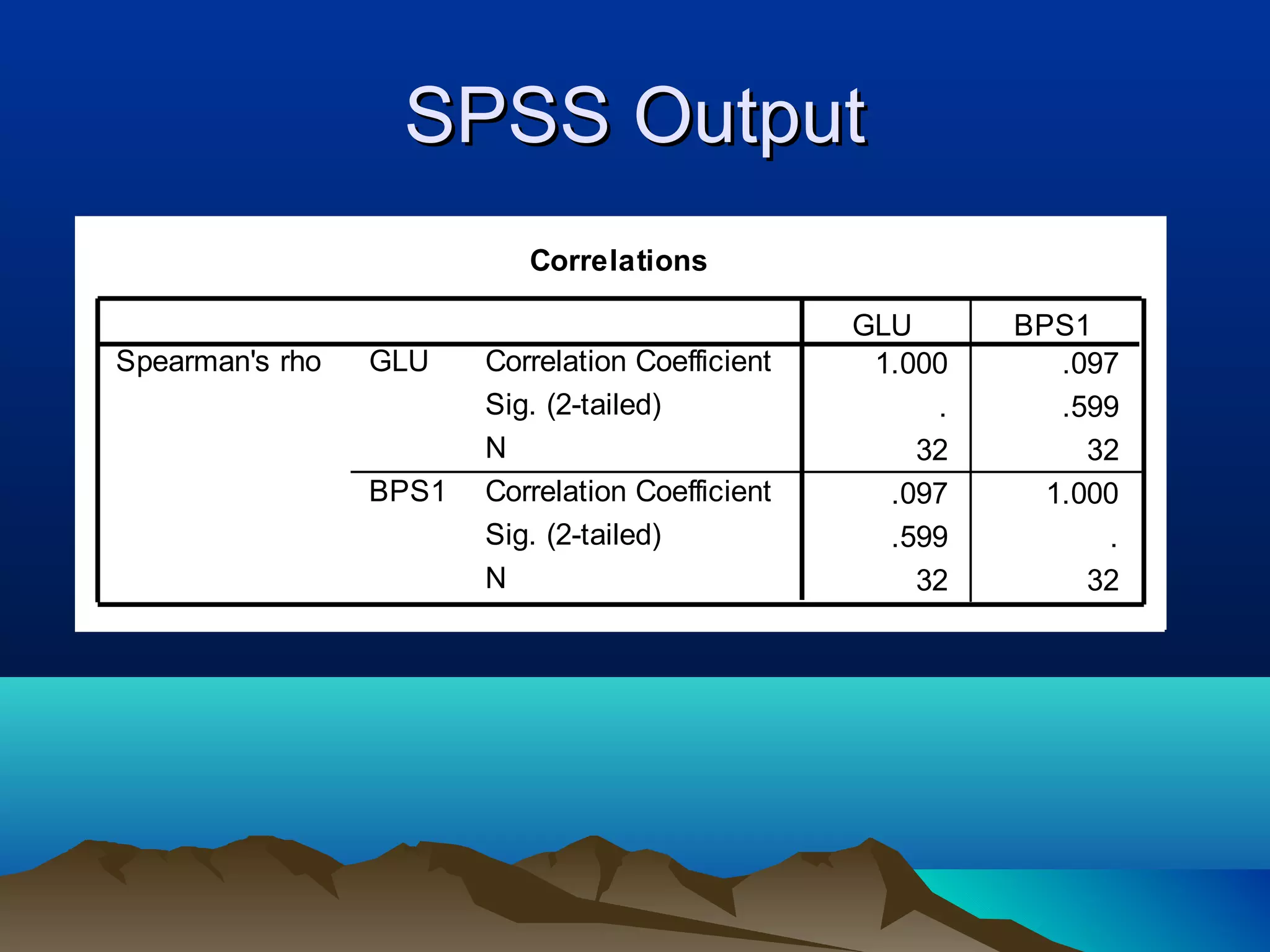

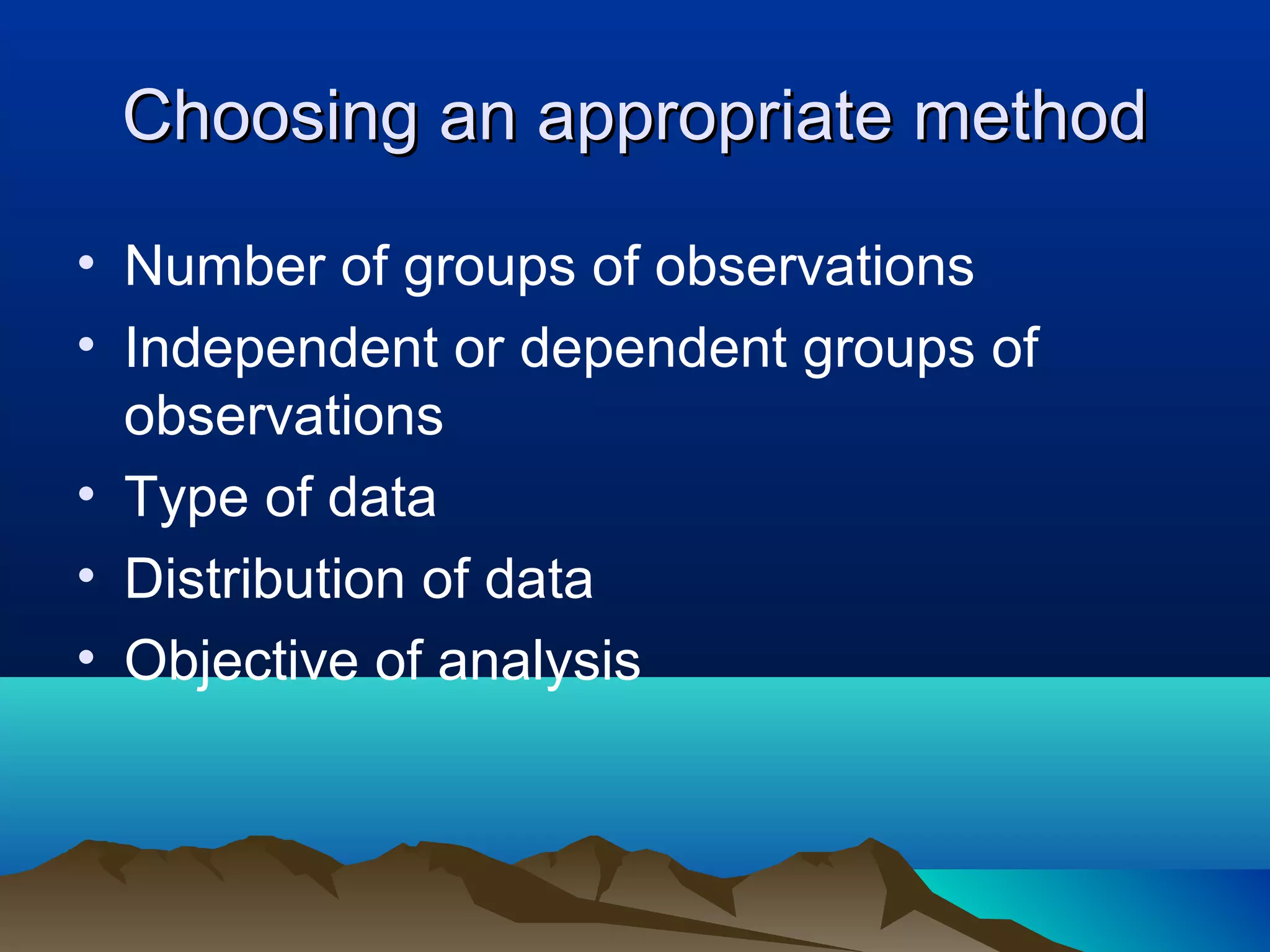
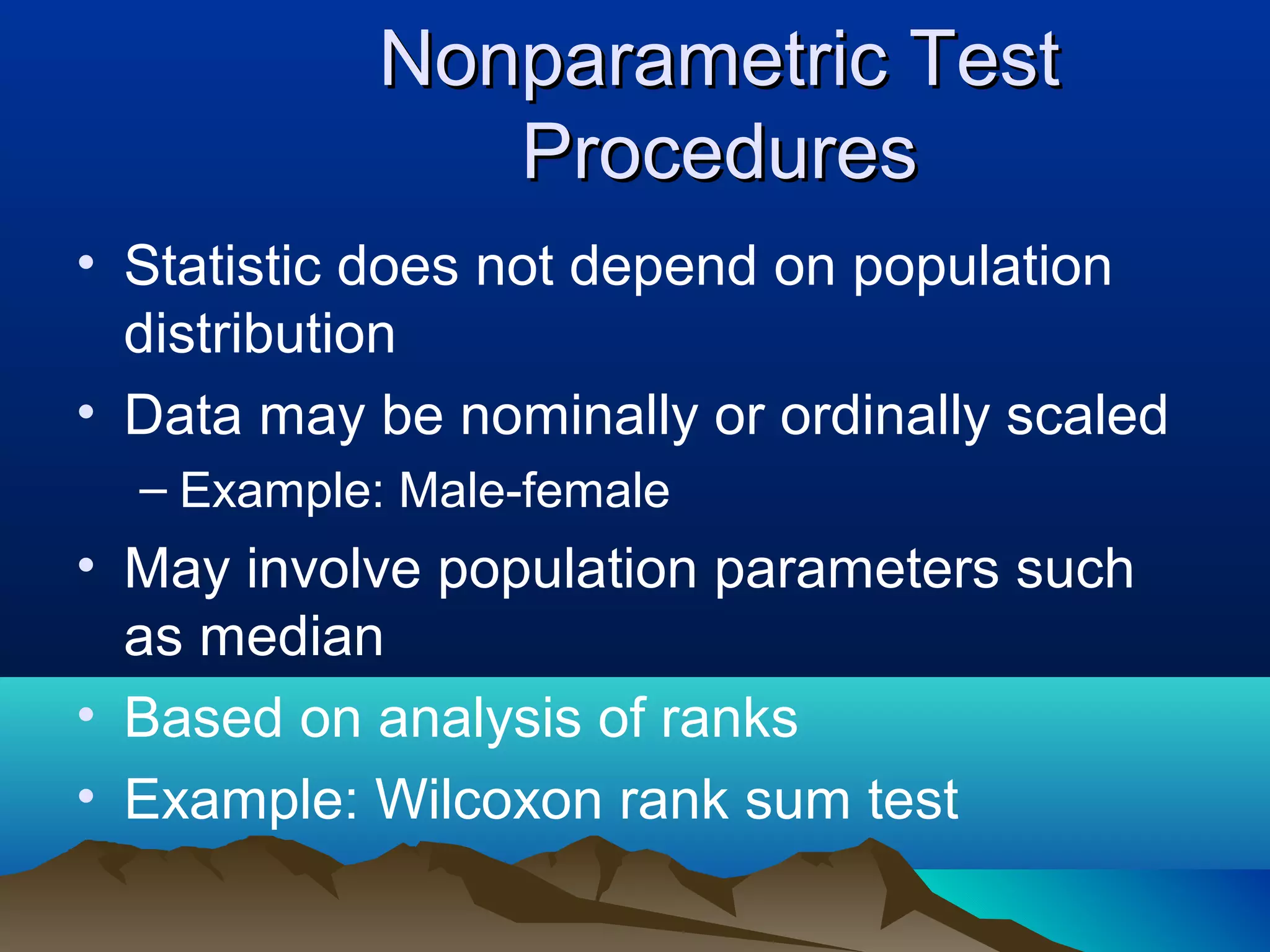
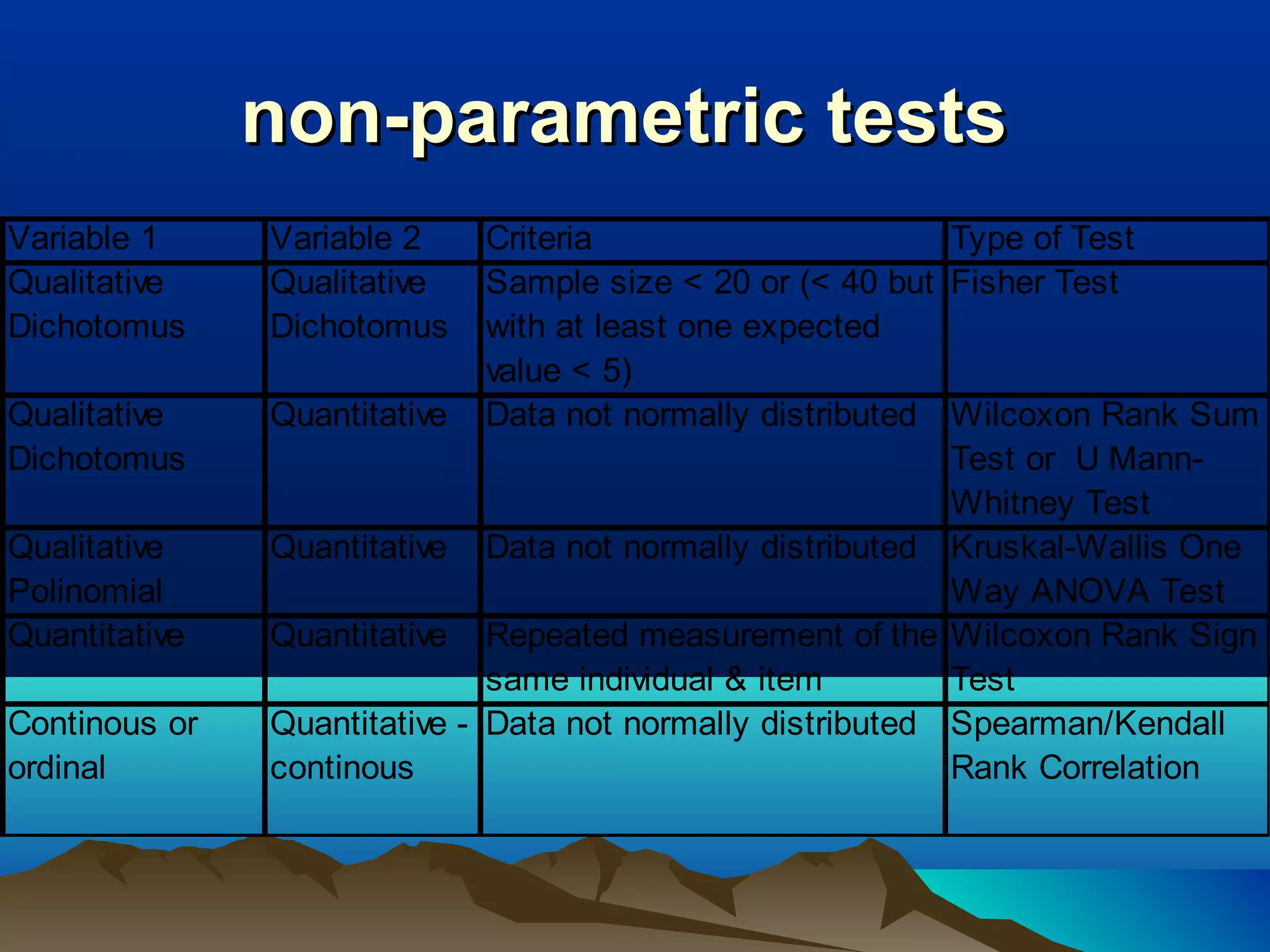
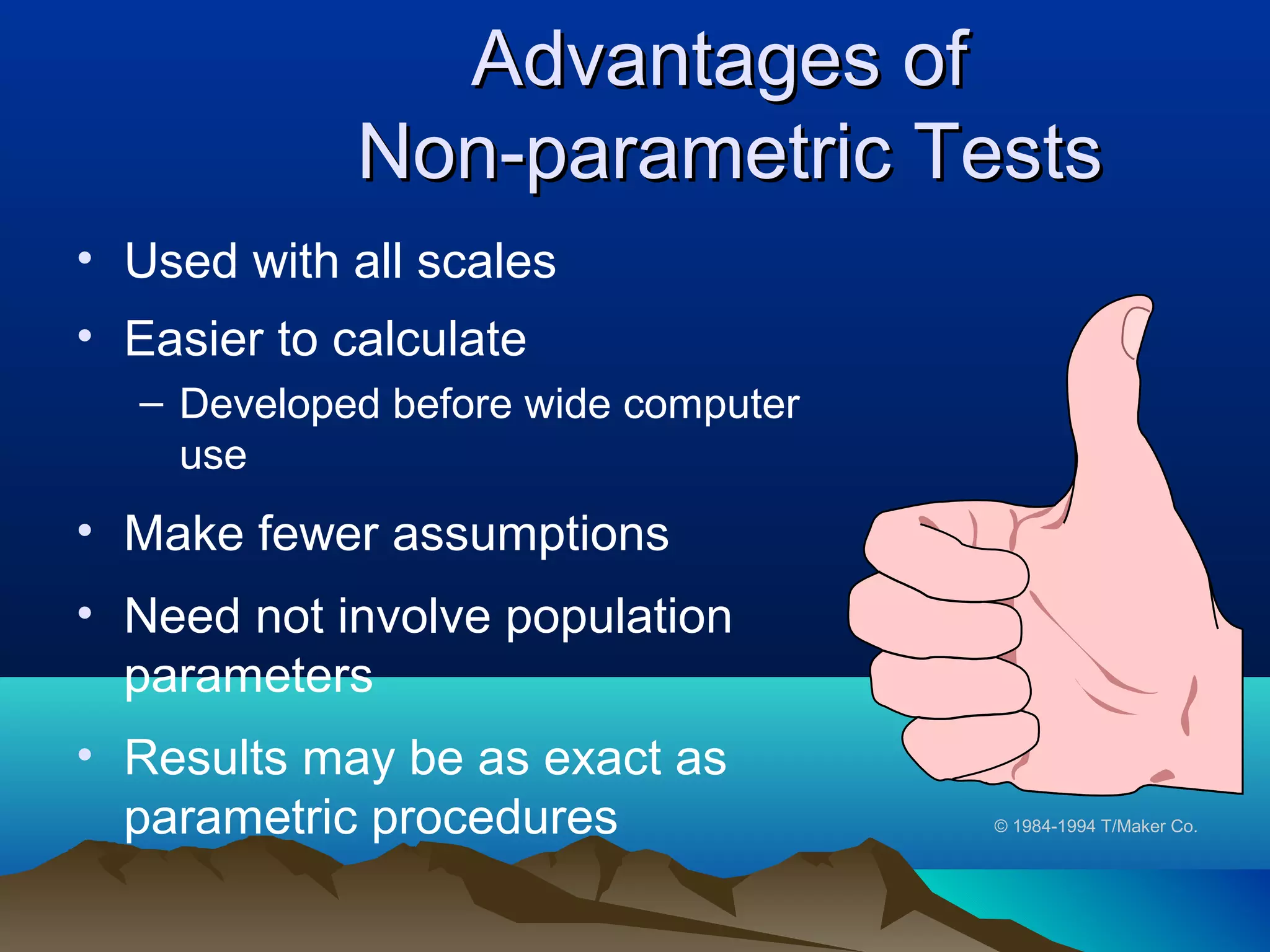
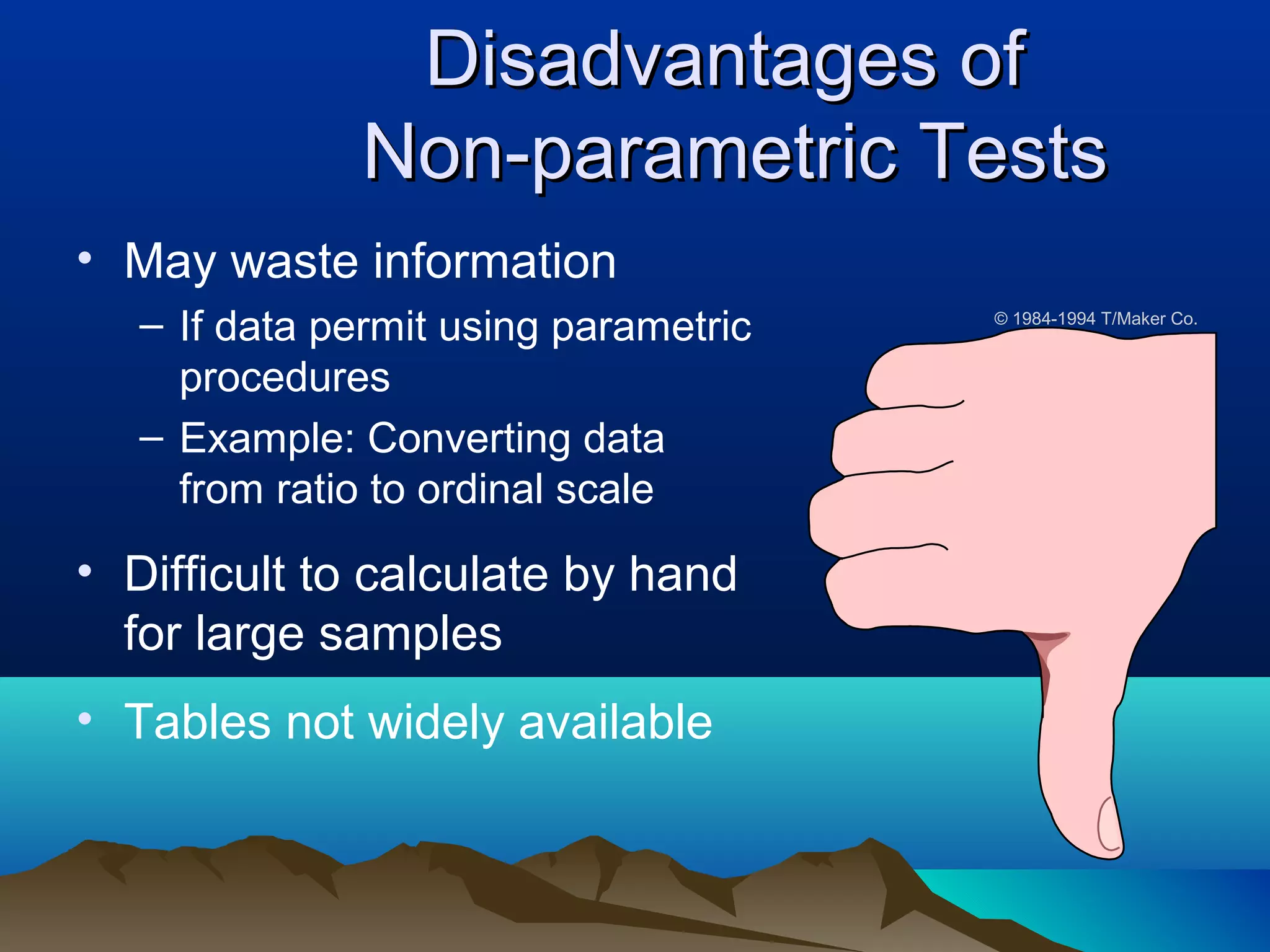
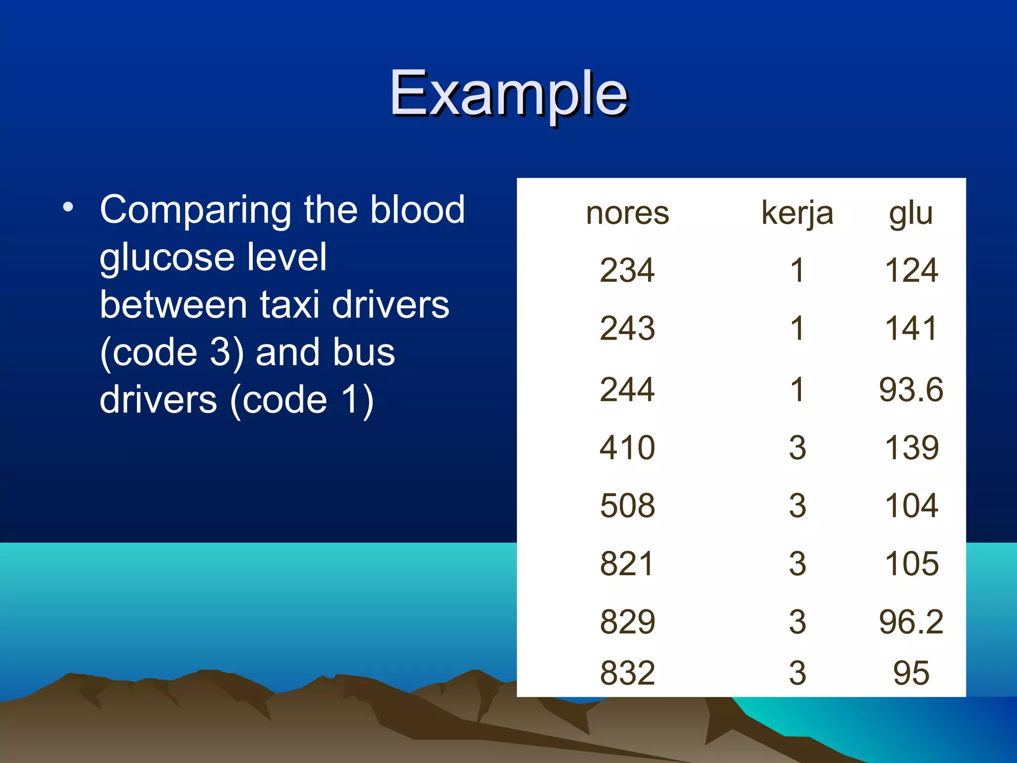
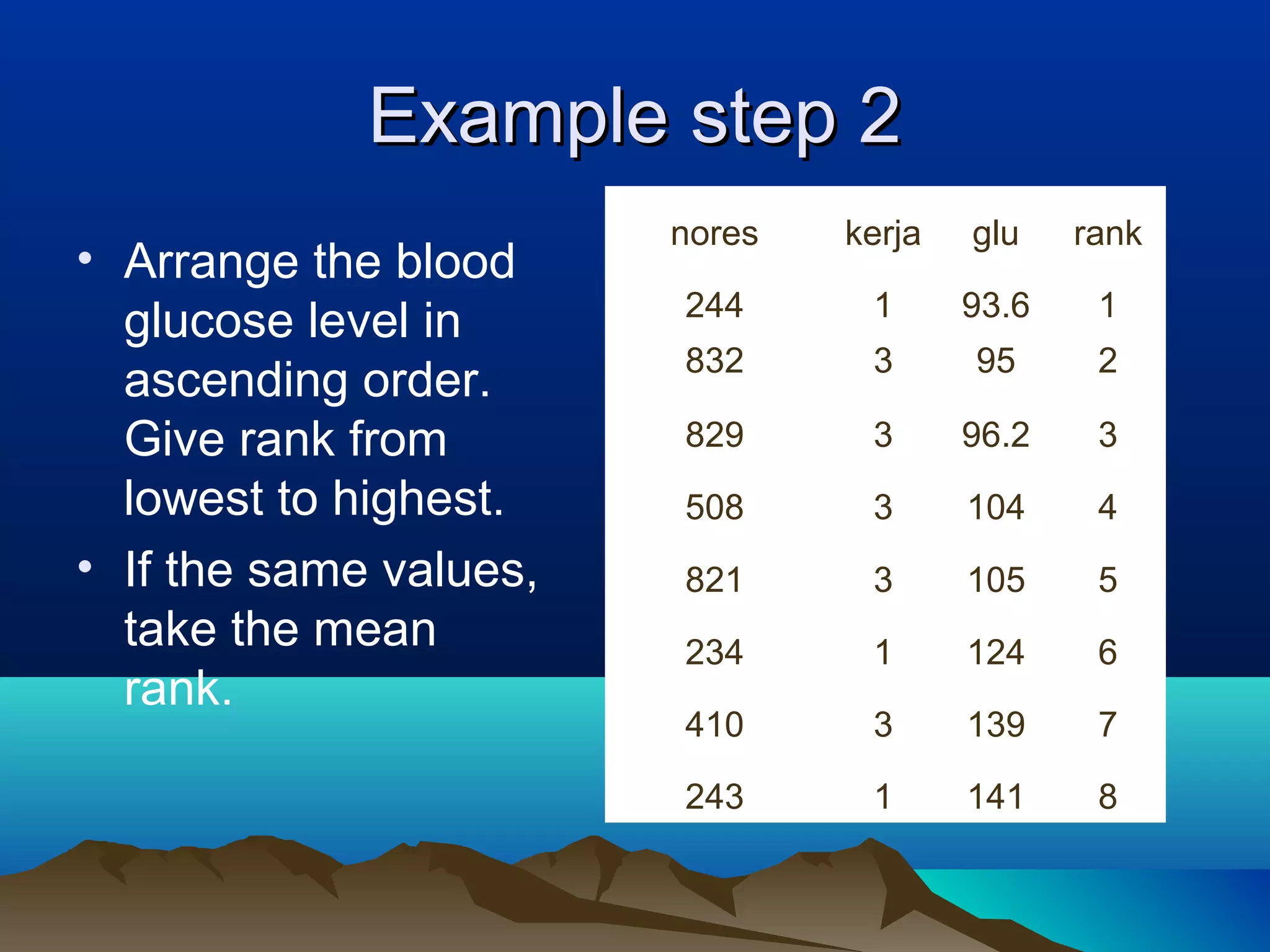
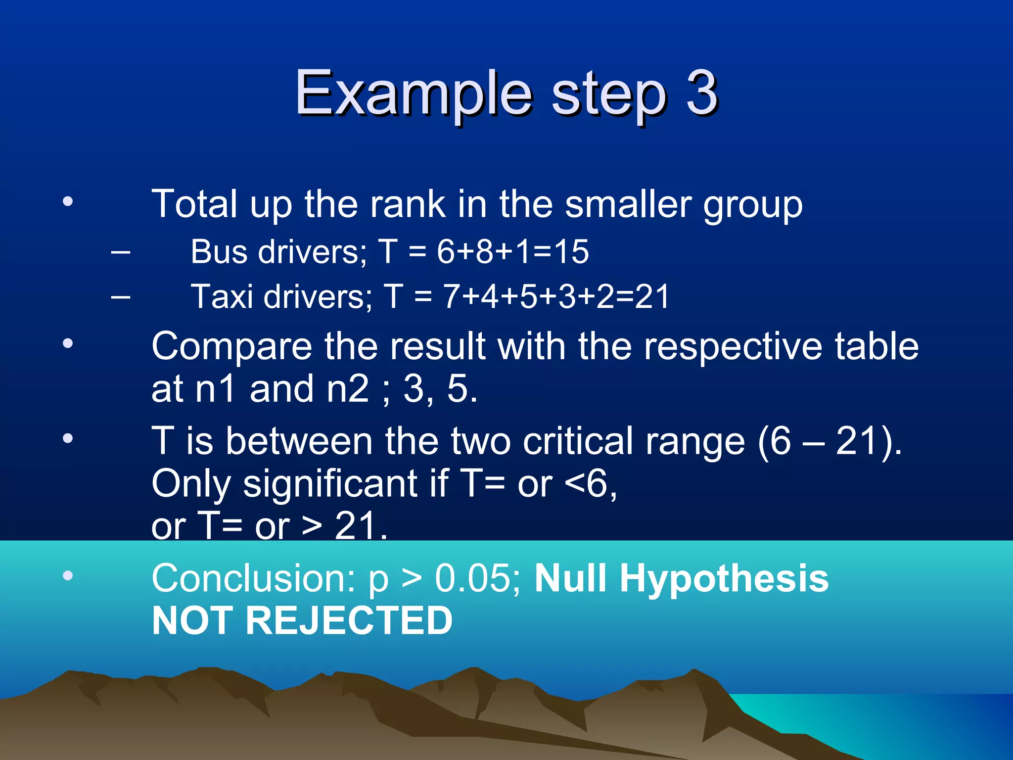
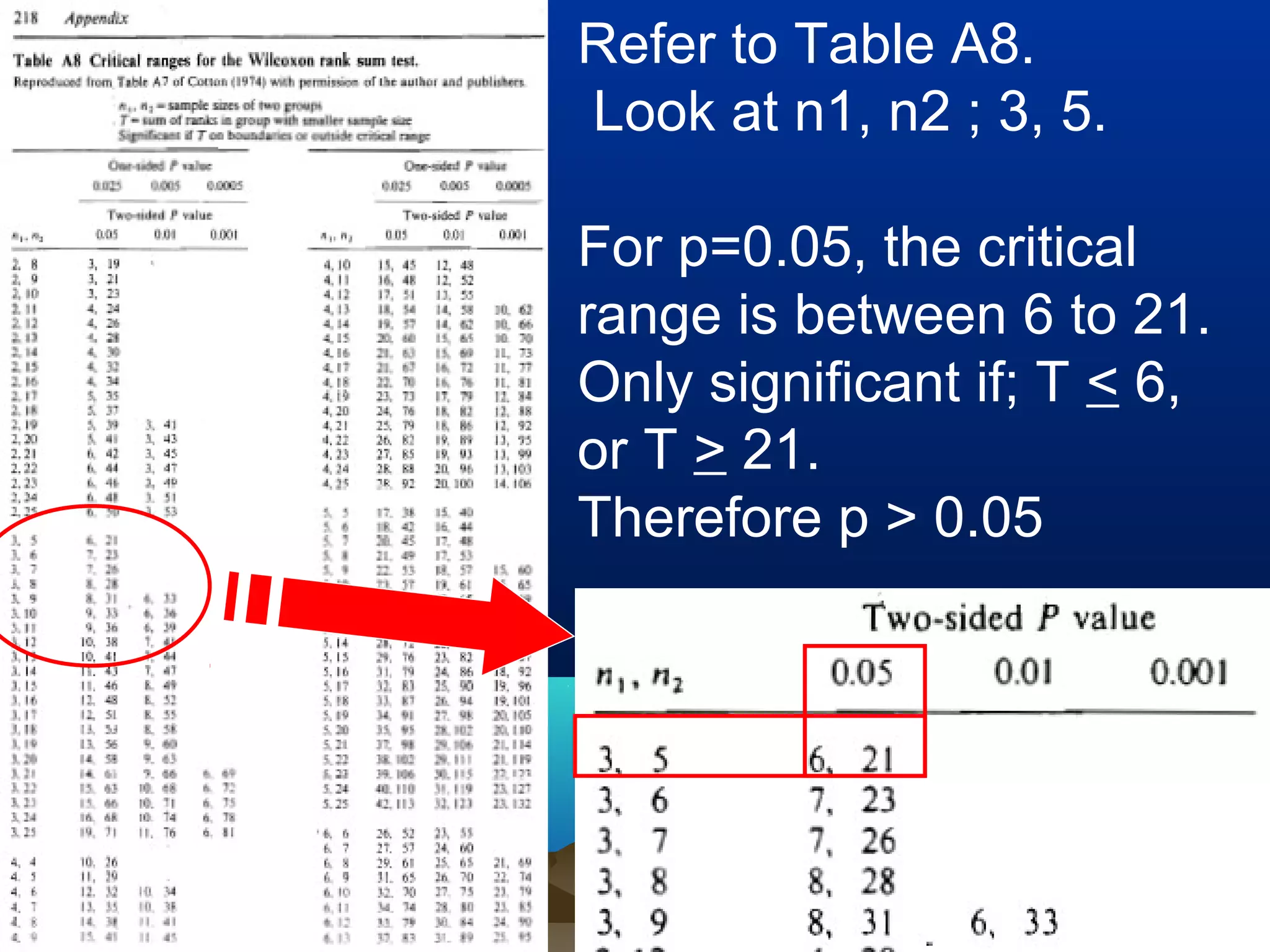
This document discusses non-parametric statistical tests including the Wilcoxon rank sum test, Kruskal-Wallis test, and Spearman/Kendall correlation. It provides an overview of when to use these tests, their assumptions, procedures, advantages and disadvantages. Examples are given to illustrate how to perform the Wilcoxon rank sum test, Kruskal-Wallis test, and Wilcoxon signed rank test step-by-step. SPSS output is also shown for these tests.