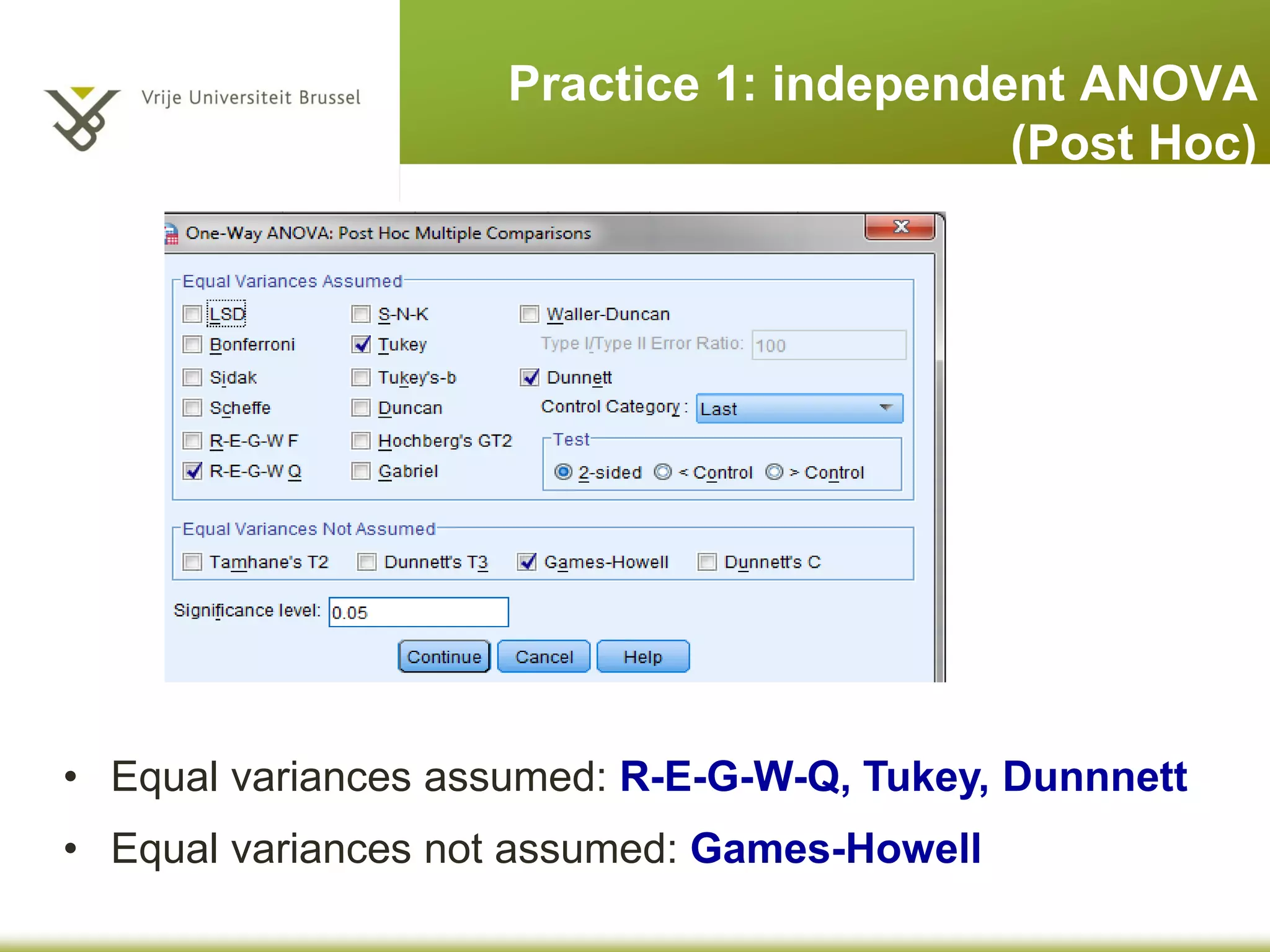
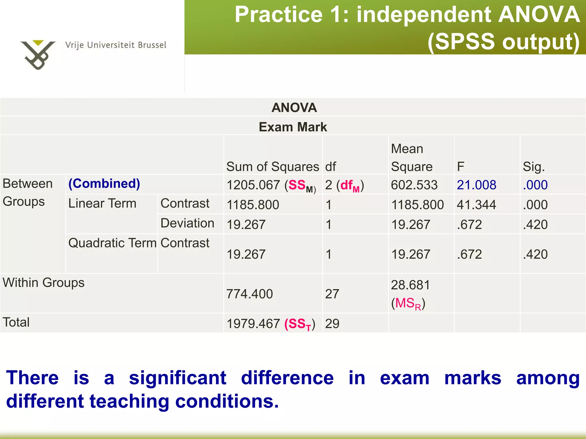
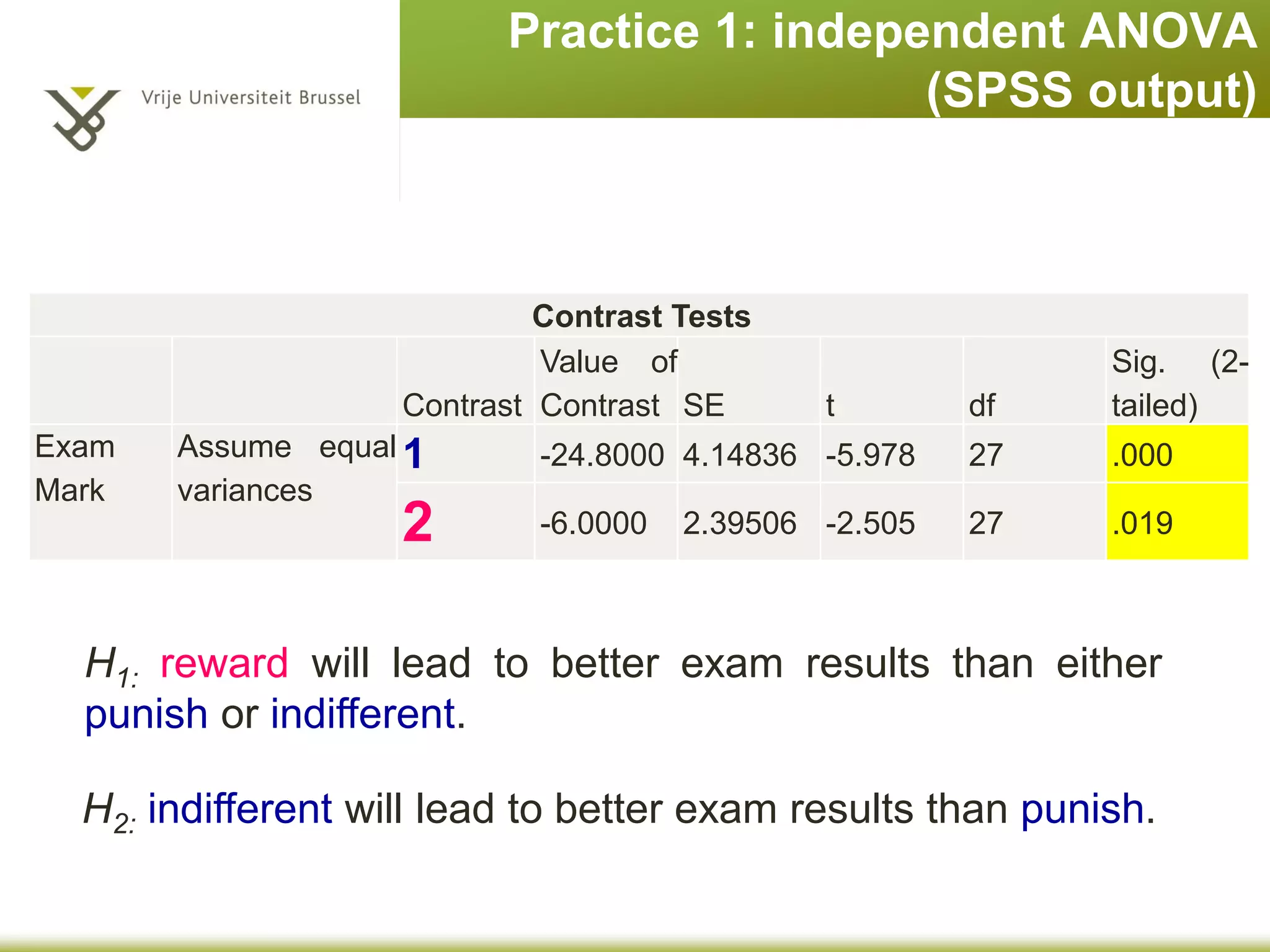
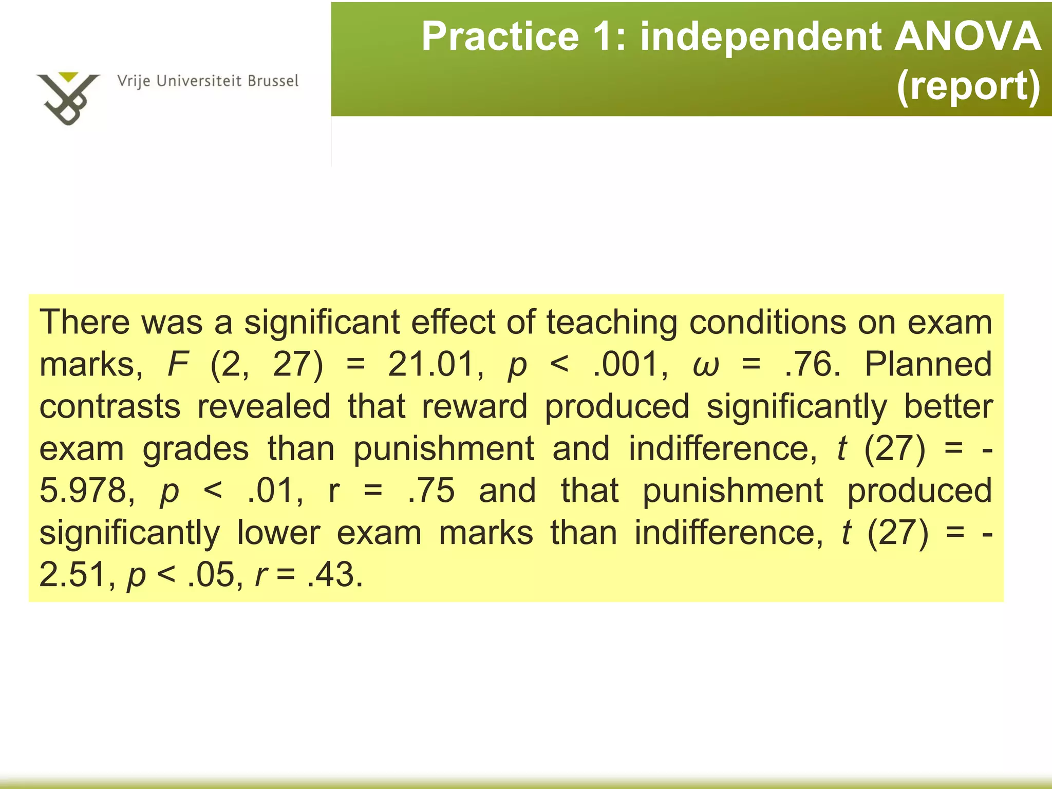
Download as PDF, PPTX


![Interpretation of the output
• Effect size
– Partial Eta Squared: the proportion of the variance in the
DV that can be explained by the IV (see Cohen, 1988)
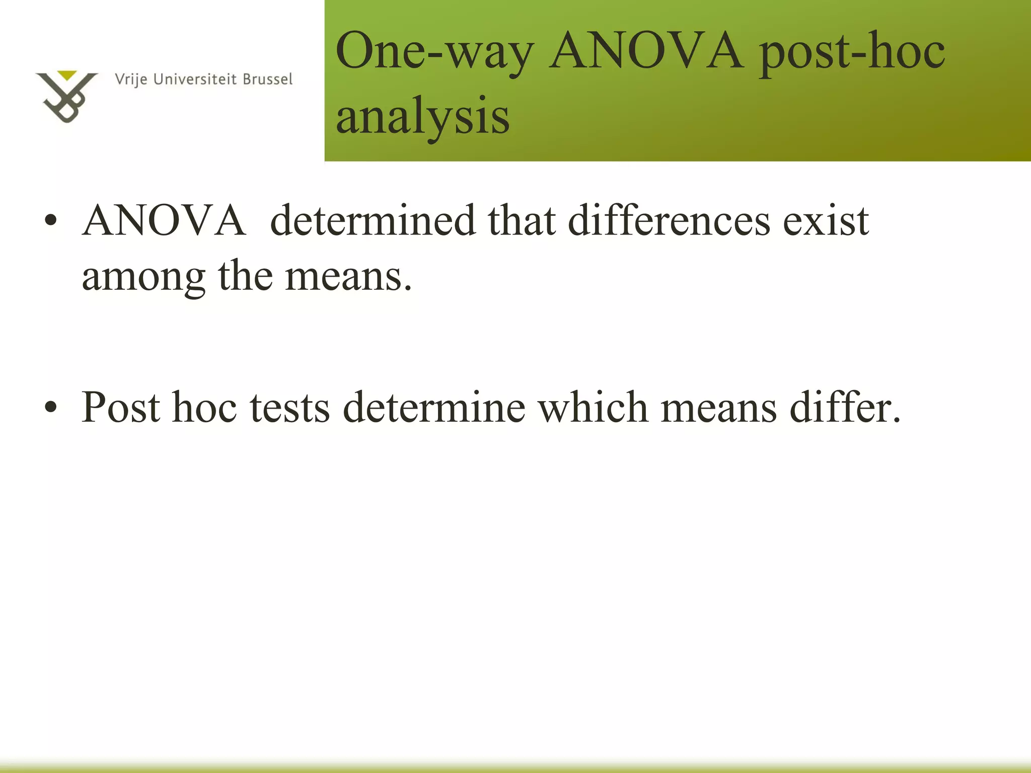
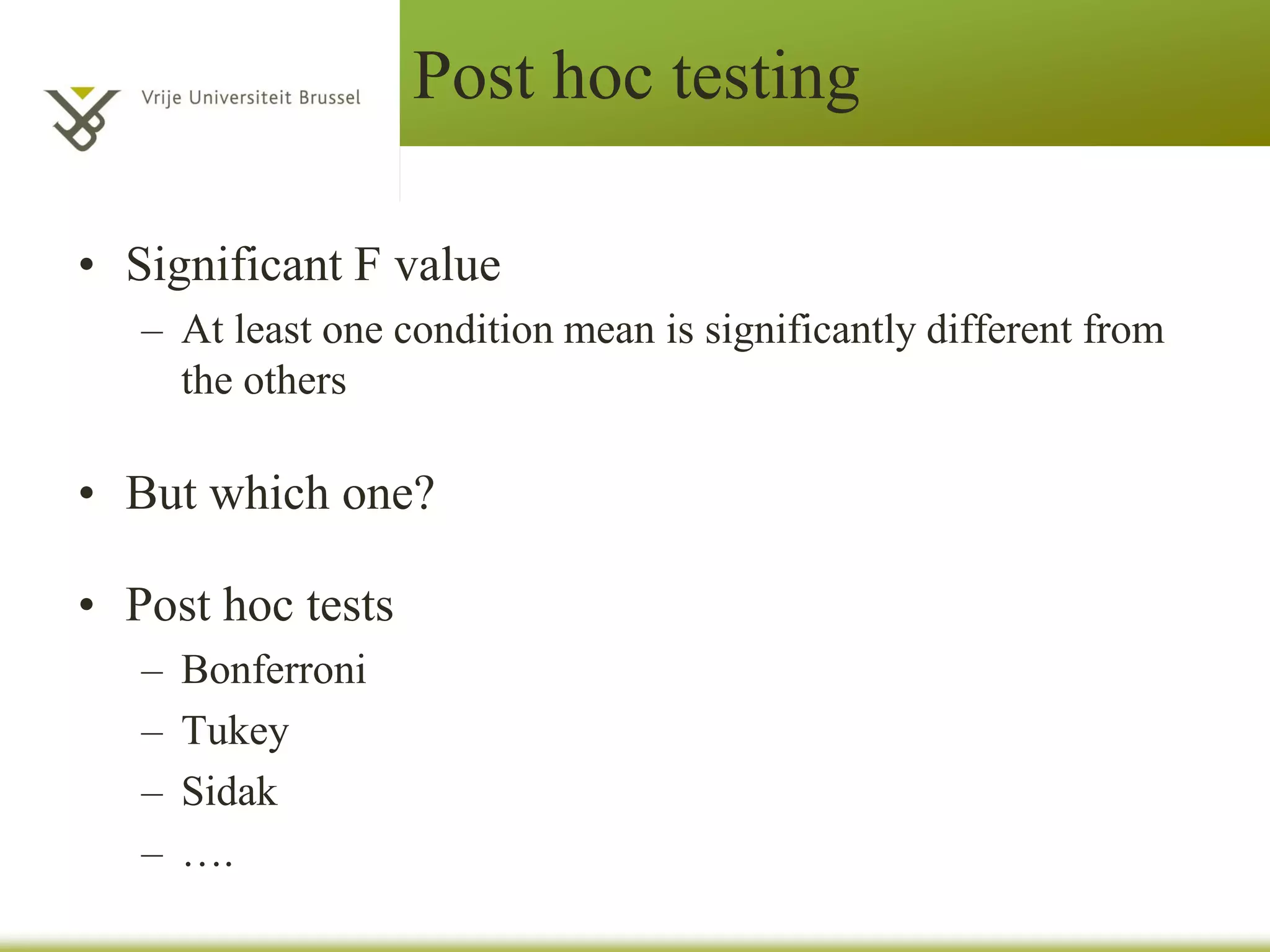
• Comparing group means
– Estimated marginal means
• Follow-up analyses
(see Hair et al., 1998; Weinfurt, 1995)
Weinfurt, K. P. (1995). Multivariate analysis of variance.
In L. G. Grimm, & P. R. Yarnold (Eds.), Reading and understanding multivariate
statistics. Washington, DC: APA. [QA278 .R43 1995]](https://image.slidesharecdn.com/appliedstatisticslecture8-150607110101-lva1-app6892/75/Applied-statistics-lecture_8-40-2048.jpg)


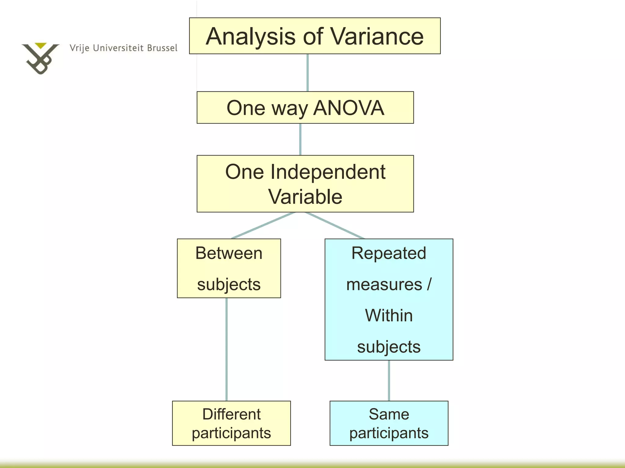
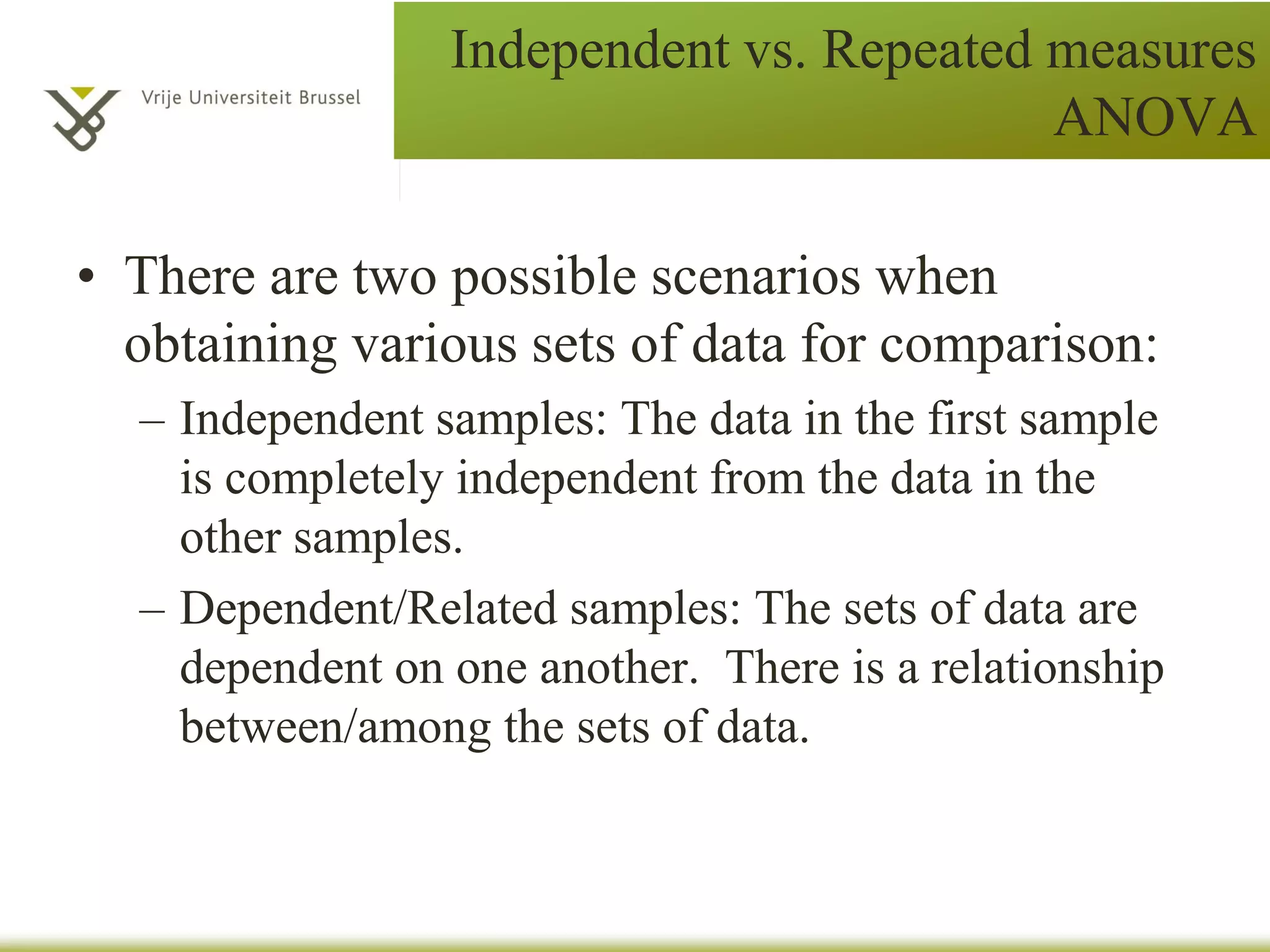
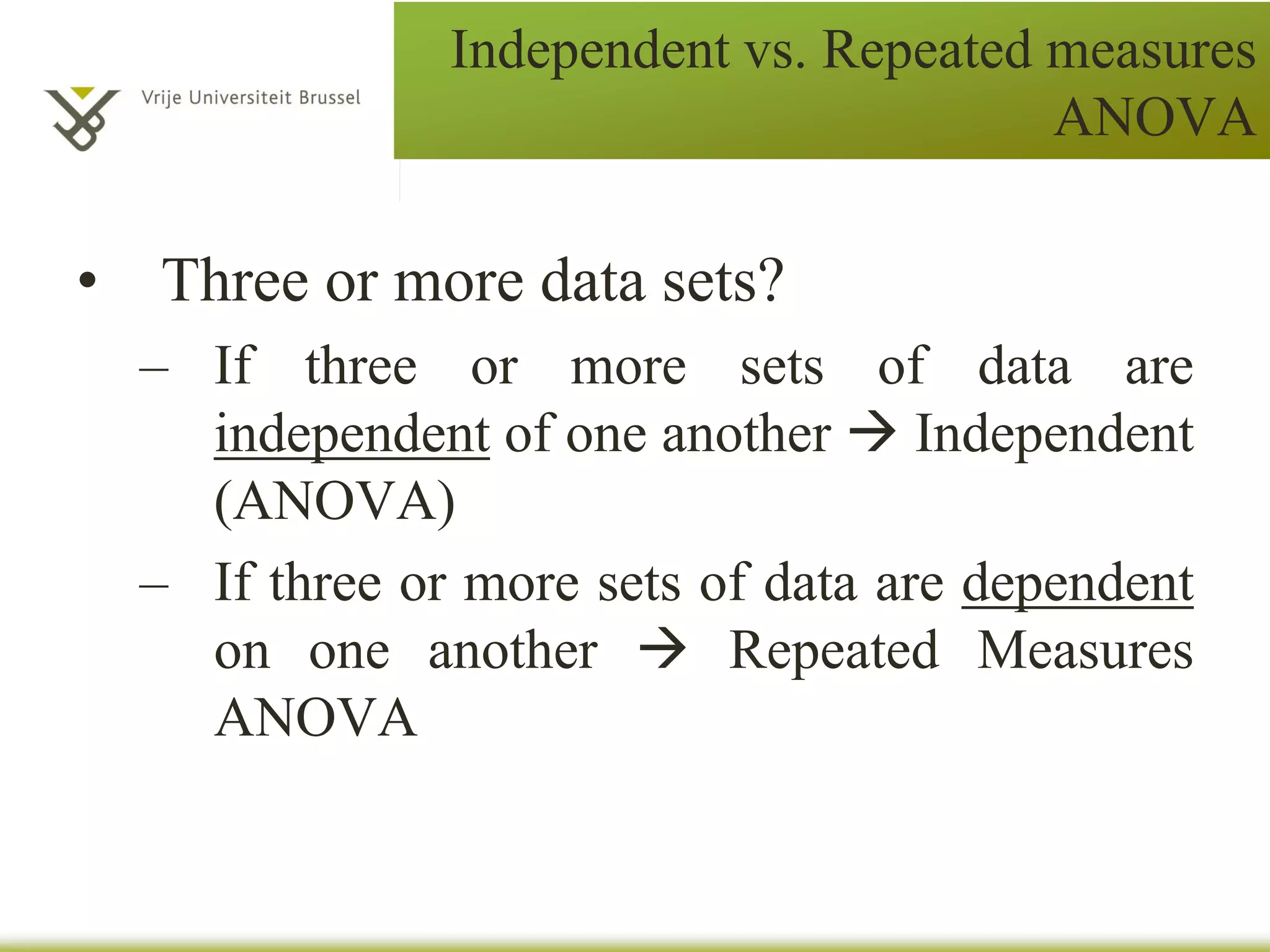
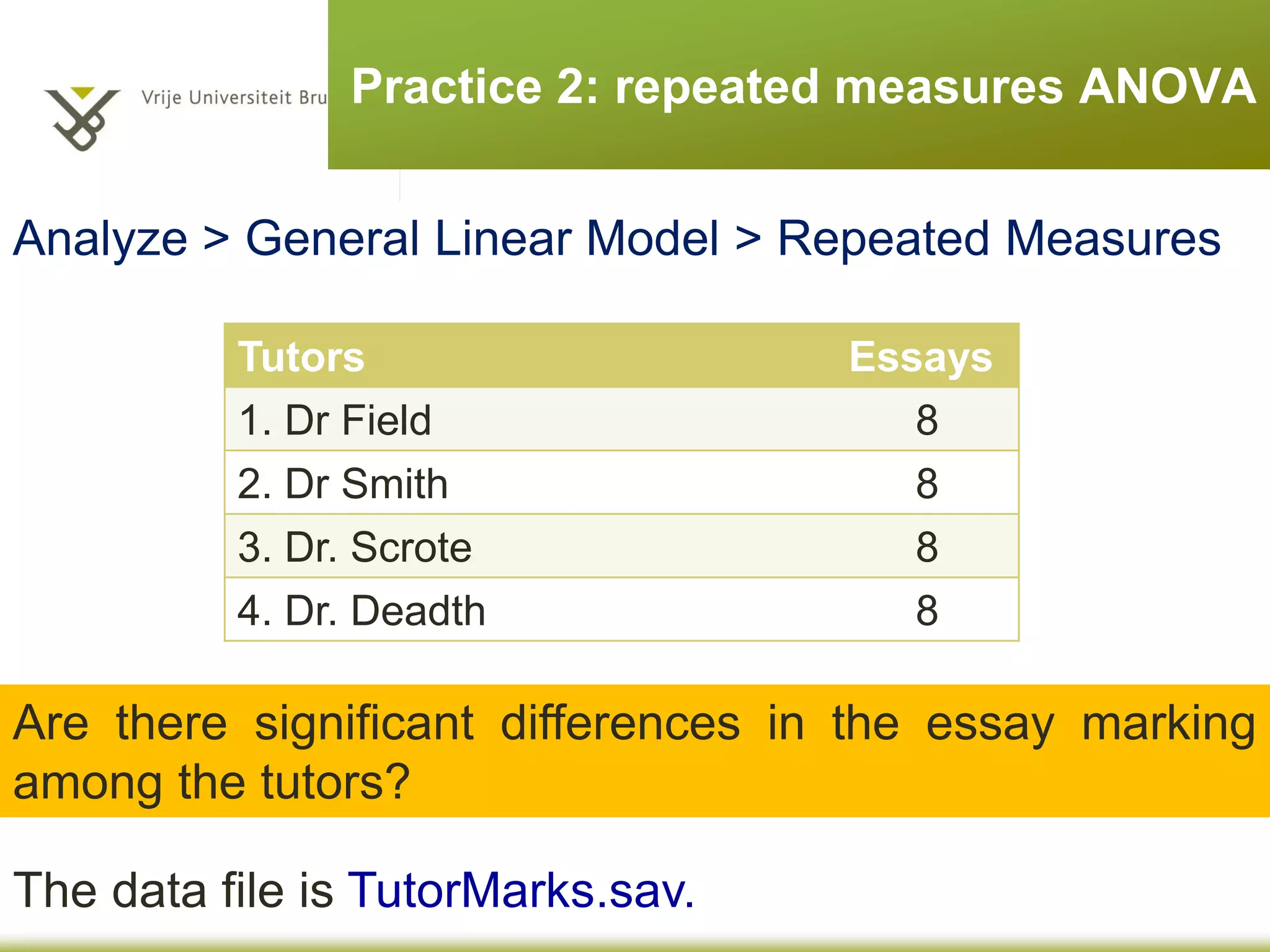
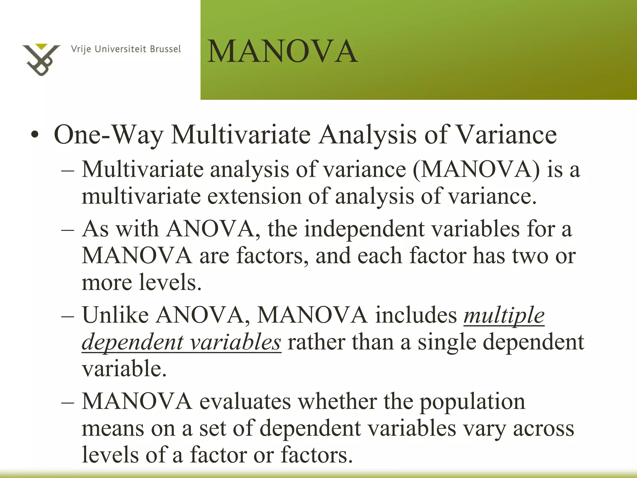
The document provides an overview of different statistical analysis methods including independent ANOVA, repeated measures ANOVA, and MANOVA. It discusses key aspects of each method such as their appropriate uses, assumptions, and how to conduct the analyses and interpret results in SPSS. For ANOVA, it covers topics like F-ratio, significance levels, post-hoc tests, effect sizes, and examples. For MANOVA, it compares it to ANOVA and explains how MANOVA can assess differences across groups on multiple dependent variables simultaneously.