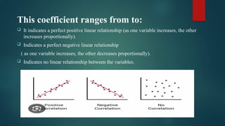
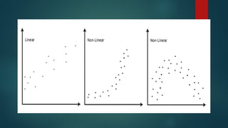
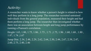
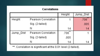
Pearson's product-moment correlation coefficient measures the strength and direction of the association between two continuous variables on at least an interval scale, indicating positive, negative, or no linear relationships. It requires data to meet four assumptions: measurement at the interval or ratio level, linearity of relationship, absence of significant outliers, and approximate normal distribution. The document also includes examples of using Pearson's correlation to assess relationships between height and long jump performance, as well as study hours and exam scores.

1. Pearson's Product-Moment
Correlation Coefficient

2. The Pearson product-moment correlation
coefficient (Pearson’s correlation, for
short) is a measure of the strength and
direction of association that exists
between two variables measured on at
least an interval scale.

3. The Pearson, or Pearson correlation
coefficient, is a statistical measure that
quantifies the strength and direction of a
linear relationship between two
continuous variables. Named after Karl
Pearson.

4. This coefficient ranges from to:
 It indicates a perfect positive linear relationship (as one variable increases, the other
increases proportionally).
 Indicates a perfect negative linear relationship
( as one variable increases, the other decreases proportionally).
 Indicates no linear relationship between the variables.

5. For example, you could use a Pearson’s
correlation to understand whether there is an
association between exam performance and
time spent revising. You could also use a
Pearson's correlation to understand whether
there is an association between depression
and length of unemployment.

6. If one of your two variables is
dichotomous you can use a point-
biserial correlation instead, or if you
have one or more control variables, you
can run a Pearson's partial correlation.

7. When you choose to analyse your data using
Pearson’s correlation, part of the process involves
checking to make sure that the data you want to
analyse can actually be analysed using Pearson’s
correlation. You need to do this because it is only
appropriate to use Pearson’s correlation if your
data "passes" four assumptions that are required
for Pearson’s correlation to give you a valid result.

8. Assumption #1:
Your two variables should be measured at the
interval or ratio level (i.e., they are continuous).
Examples of variables that meet this criterion
include revision time (measured in hours),
intelligence (measured using IQ score), exam
performance (measured from 0 to 100), weight
(measured in kg), and so forth.

9. Assumption #2: There is a linear
relationship between your two
variables. Whilst there are a number of
ways to check whether a linear
relationship exists between your two
variables,

11. If the relationship displayed in your scatterplot is
not linear, you will have to either run a
nonparametric equivalent to Pearson’s correlation
or transform your data, which you can do using
SPSS Statistics.

12. Pearson's correlation determines the degree to which a relationship is linear.
Put another way, it determines whether there is a linear component of
association between two continuous variables. As such, linearity is not actually
an assumption of Pearson's correlation. However, you would not normally
want to pursue a Pearson's correlation to determine the strength and direction
of a linear relationship when you already know the relationship between your
two variables is not linear. Instead, the relationship between your two variables
might be better described by another statistical measure. For this reason, it is
not uncommon to view the relationship between your two variables in a
scatterplot to see if running a Pearson's correlation is the best choice as a
measure of association or whether another measure would be better.

13. Assumption #3:
There should be no significant outliers. Outliers are
simply single data points within your data that do not
follow the usual pattern (e.g., in a study of 100 students’
IQ scores, where the mean score was 108 with only a
small variation between students, one student had a score
of 156, which is very unusual, and may even put her in
the top 1% of IQ scores globally). The following
scatterplots highlight the potential impact of outliers:

15. Pearson’s correlation coefficient, r, is
sensitive to outliers, which can have a very
large effect on the line of best fit and the
Pearson correlation coefficient. Therefore, in
some cases, including outliers in your
analysis can lead to misleading results.
Therefore, it is best if there are no outliers or
they are kept to a minimum.

16. Assumption #4:
Your variables should be approximately normally
distributed. In order to assess the statistical significance
of the Pearson correlation, you need to have bivariate
normality, but this assumption is difficult to assess, so a
simpler method is more commonly used. This simpler
method involves determining the normality of each
variable separately. To test for normality you can use the
Shapiro-Wilk test of normality, which is easily tested for
using SPSS Statistics.

17. Activity:
A researcher wants to know whether a person's height is related to how
well they perform in a long jump. The researcher recruited untrained
individuals from the general population, measured their height and had
them perform a long jump. The researcher then investigated whether
there was an association between height and long jump performance by
running a Pearson's correlation.
Height 1.63, 1.80, 1.75, 1.86 , 1.73 , 1.71 ,1.75, 1.96 , 1.60, 1.68 , 1.80 ,
1.87, 1.74 ,1.67
Jump Dist. 2.34, 2.48, 2.29, 2.62, 2.64, 2.30, 2.44, 2.67, 2.39, 2.47,
2.60, 2.75, 2.40, 2.46

23. Activity:
A researcher wants to know if there is a relationship between the
number of hours a student studies for an exam and their exam score.
They collected data from a group of students, recording the number
of hours each student studied and their corresponding exam score.
Hours Studied: 2, 3, 4, 5, 6, 7, 8, 9, 10
Exam Score: 60, 65, 70, 75, 80, 85, 90, 95, 100,100