Download as PDF, PPTX
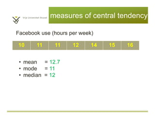
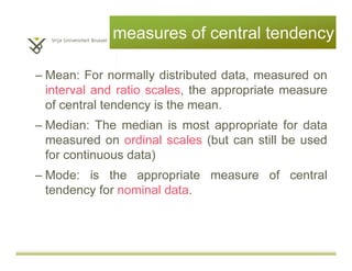
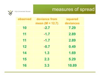
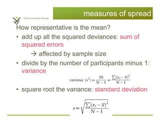
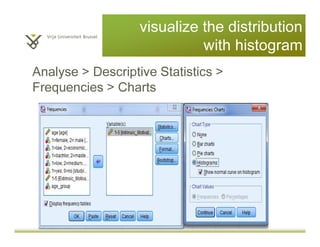
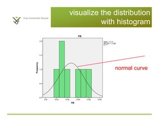
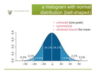
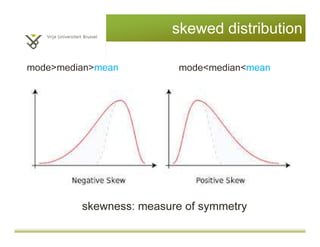
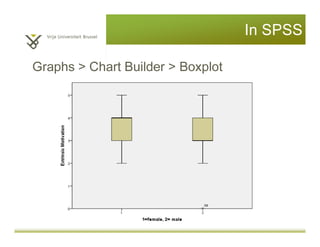
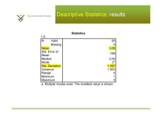
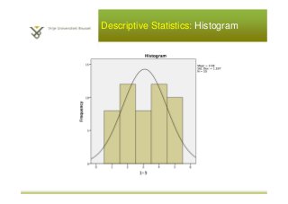
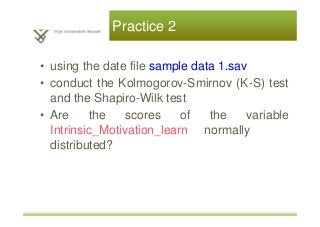
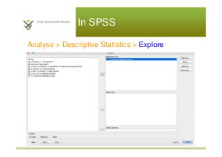
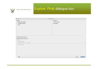

This document provides an introduction to descriptive statistics and statistical methods. It discusses the aims of exploring data through descriptive statistics like measures of central tendency (mean, median, mode) and dispersion (range, variance, standard deviation). It also covers testing assumptions like normal distribution through histograms and statistical tests. Examples are provided to demonstrate calculating and interpreting these descriptive statistics in SPSS. Practices are included to have the reader conduct descriptive analyses and normality tests on sample data sets in SPSS.