A mixed between-within subjects ANOVA was conducted to examine the impact of different instruction methods (lecture, slides, instruction with student presentation, pair work) on linguistics test scores over two time periods (pretest and posttest) among 32 students randomly assigned to four groups. There was a significant interaction between time and instruction method, and time had a significant main effect. The different instruction methods also had a significant main effect on test scores. Post hoc tests revealed significant differences in scores between the lecture and student presentation groups, and the student presentation and pair work groups.

1. Mixed between-within
groups ANOVA
By Mahsa Farahanynia
PhD student
Allameh Tabataba‘i University, Iran
2015

2. Null Hypothesis
 Null hypothesis: Different methods of instruction (lecture type
instruction, present the topics using slides, given instruction
combined with student presentation, and pair work discussion of
issues) do not have a significant effect on the learners’ linguistics
achievement.

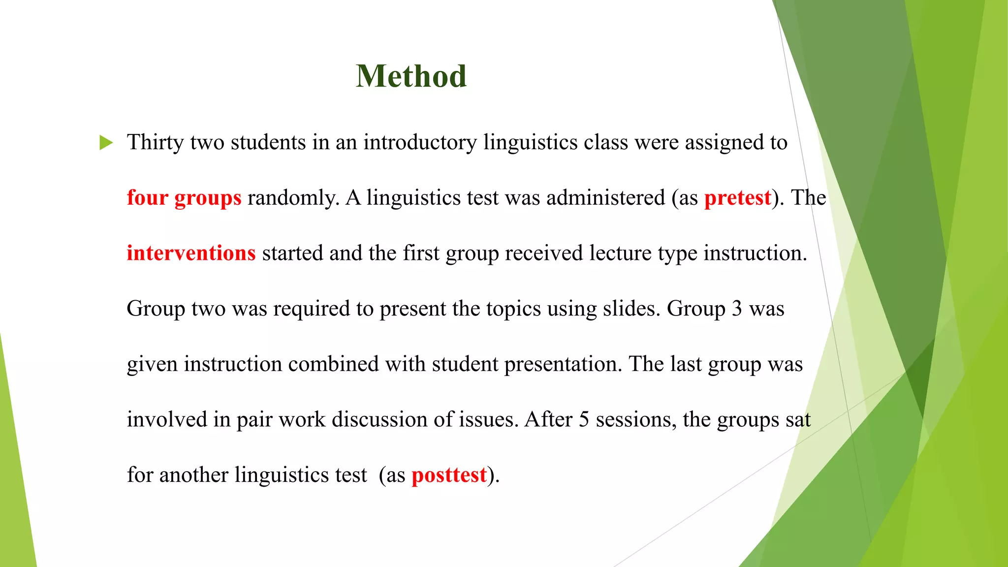
3. Method
 Thirty two students in an introductory linguistics class were assigned to
four groups randomly. A linguistics test was administered (as pretest). The
interventions started and the first group received lecture type instruction.
Group two was required to present the topics using slides. Group 3 was
given instruction combined with student presentation. The last group was
involved in pair work discussion of issues. After 5 sessions, the groups sat
for another linguistics test (as posttest).

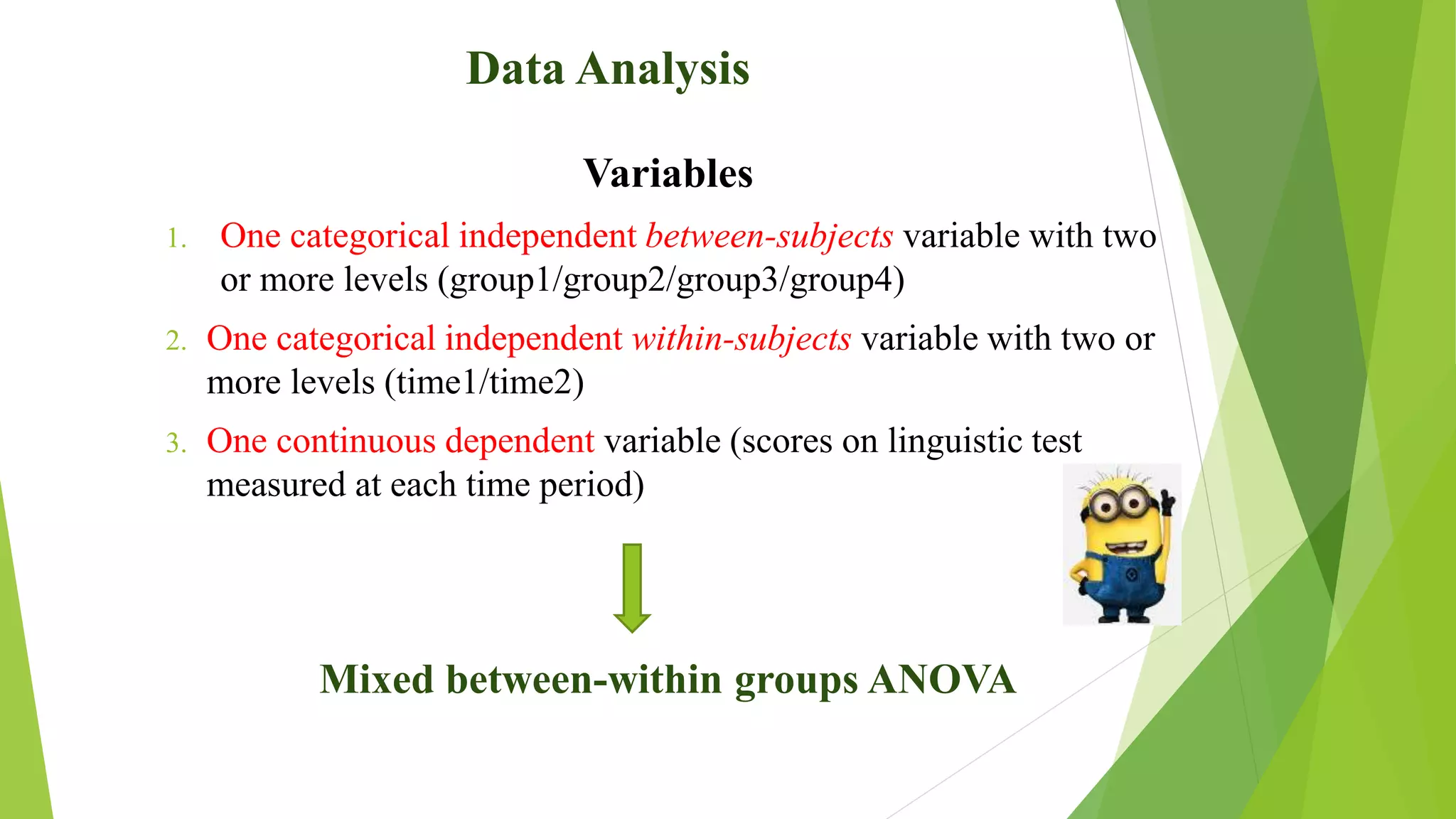
4. Data Analysis
Variables
1. One categorical independent between-subjects variable with two
or more levels (group1/group2/group3/group4)
2. One categorical independent within-subjects variable with two or
more levels (time1/time2)
3. One continuous dependent variable (scores on linguistic test
measured at each time period)
Mixed between-within groups ANOVA

5. Step 1: Normality of the data
Analyze explore

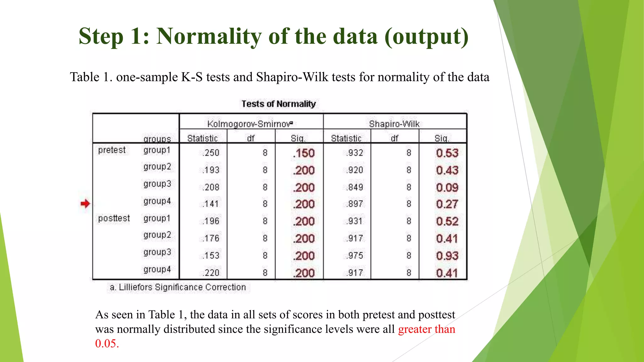
6. Step 1: Normality of the data (output)
Table 1. one-sample K-S tests and Shapiro-Wilk tests for normality of the data
As seen in Table 1, the data in all sets of scores in both pretest and posttest
was normally distributed since the significance levels were all greater than
0.05.

7. Mixed between-within groups ANOVA in SPSS
 Analyze General Linear Model Repeated measures

8. Mixed between-within groups ANOVA in SPSS

9. Mixed between-within groups ANOVA in SPSS

10. Step 2: Descriptive Statistics
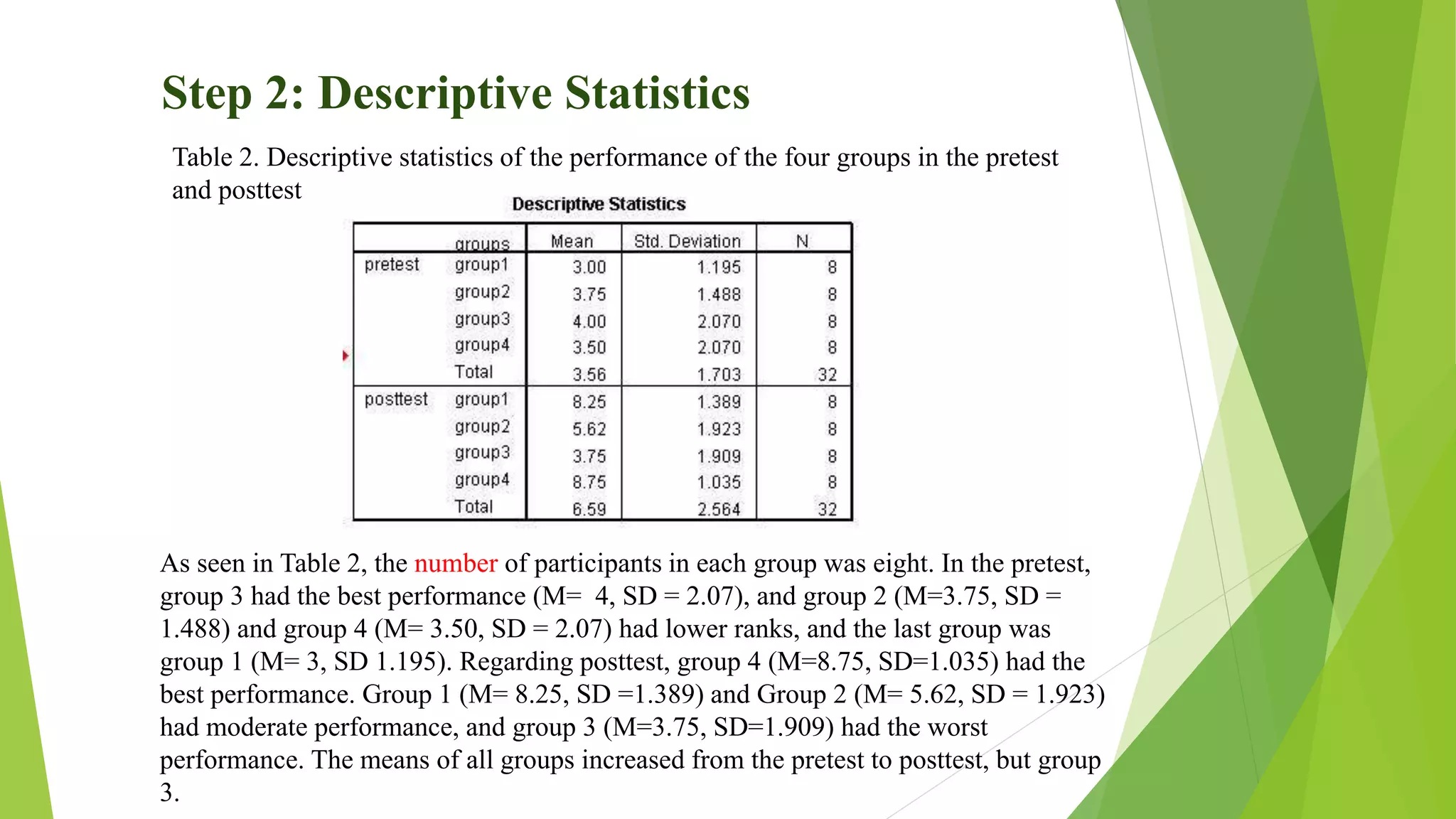
As seen in Table 2, the number of participants in each group was eight. In the pretest,
group 3 had the best performance (M= 4, SD = 2.07), and group 2 (M=3.75, SD =
1.488) and group 4 (M= 3.50, SD = 2.07) had lower ranks, and the last group was
group 1 (M= 3, SD 1.195). Regarding posttest, group 4 (M=8.75, SD=1.035) had the
best performance. Group 1 (M= 8.25, SD =1.389) and Group 2 (M= 5.62, SD = 1.923)
had moderate performance, and group 3 (M=3.75, SD=1.909) had the worst
performance. The means of all groups increased from the pretest to posttest, but group
3.
Table 2. Descriptive statistics of the performance of the four groups in the pretest
and posttest

11. Step 3: Checking Assumptions
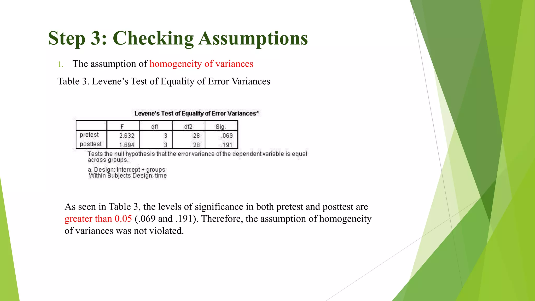
1. The assumption of homogeneity of variances
Table 3. Levene’s Test of Equality of Error Variances
As seen in Table 3, the levels of significance in both pretest and posttest are
greater than 0.05 (.069 and .191). Therefore, the assumption of homogeneity
of variances was not violated.

12. Step 3: Checking Assumptions (Cont.)
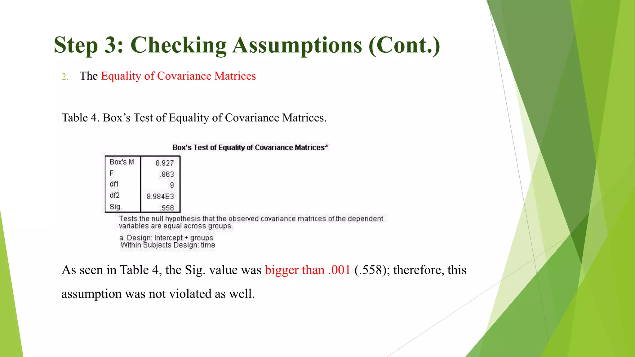
2. The Equality of Covariance Matrices
Table 4. Box’s Test of Equality of Covariance Matrices.
As seen in Table 4, the Sig. value was bigger than .001 (.558); therefore, this
assumption was not violated as well.

13. Step 4: Interaction effect and Main effect
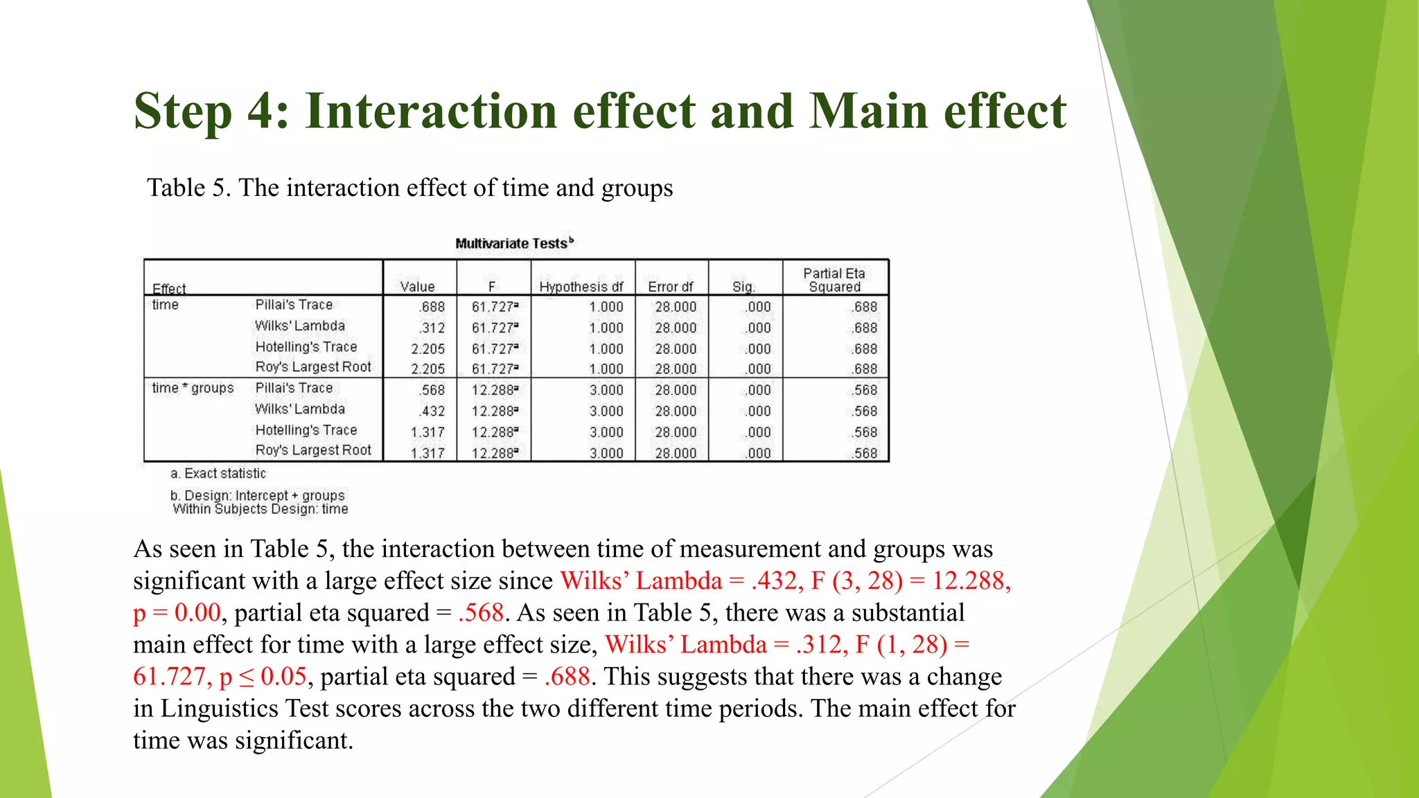
Table 5. The interaction effect of time and groups
As seen in Table 5, the interaction between time of measurement and groups was
significant with a large effect size since Wilks’ Lambda = .432, F (3, 28) = 12.288,
p = 0.00, partial eta squared = .568. As seen in Table 5, there was a substantial
main effect for time with a large effect size, Wilks’ Lambda = .312, F (1, 28) =
61.727, p ≤ 0.05, partial eta squared = .688. This suggests that there was a change
in Linguistics Test scores across the two different time periods. The main effect for
time was significant.

14. Step 5: Between-subjects effect
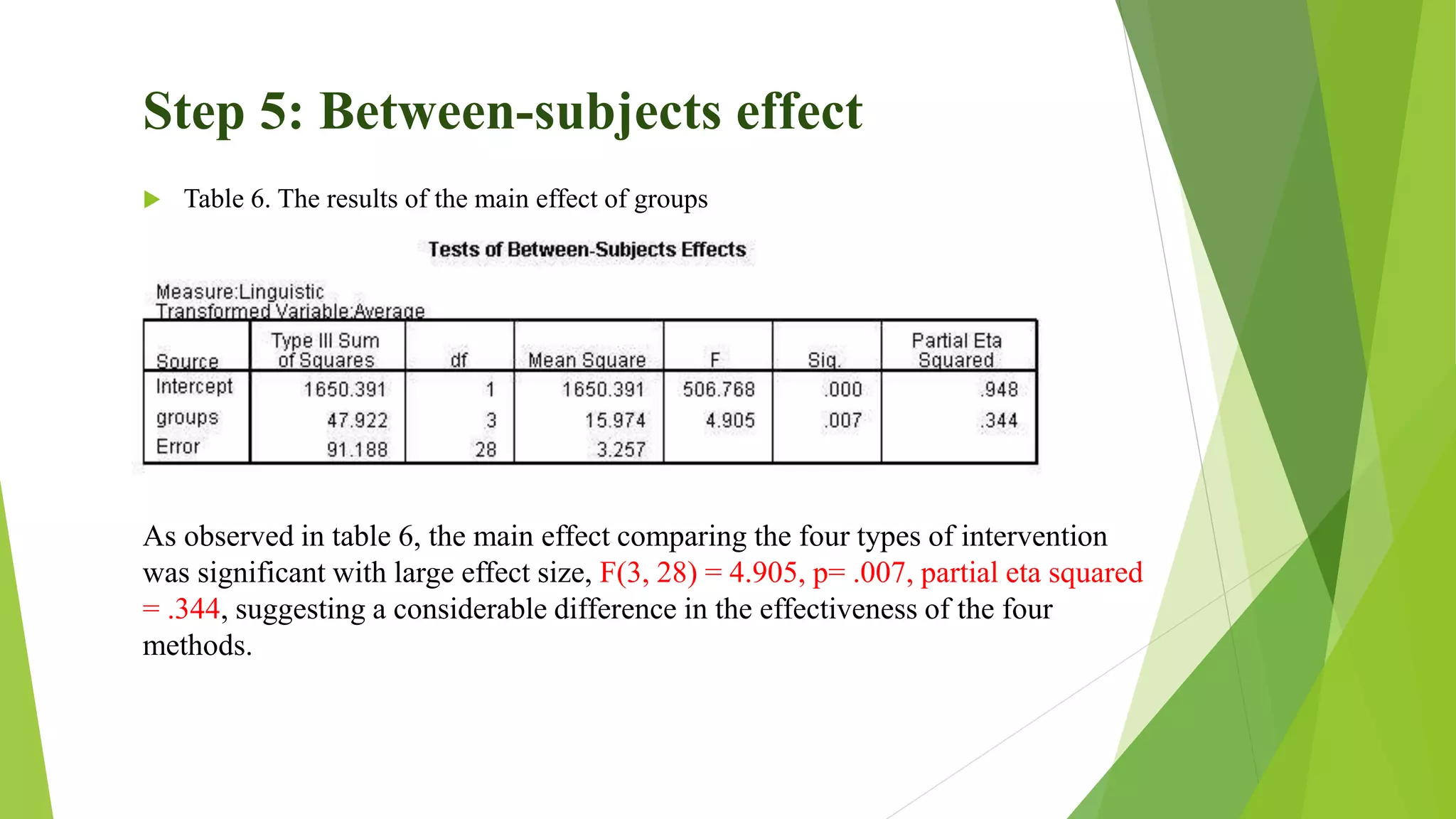
 Table 6. The results of the main effect of groups
As observed in table 6, the main effect comparing the four types of intervention
was significant with large effect size, F(3, 28) = 4.905, p= .007, partial eta squared
= .344, suggesting a considerable difference in the effectiveness of the four
methods.

15. Step 6: Post hoc
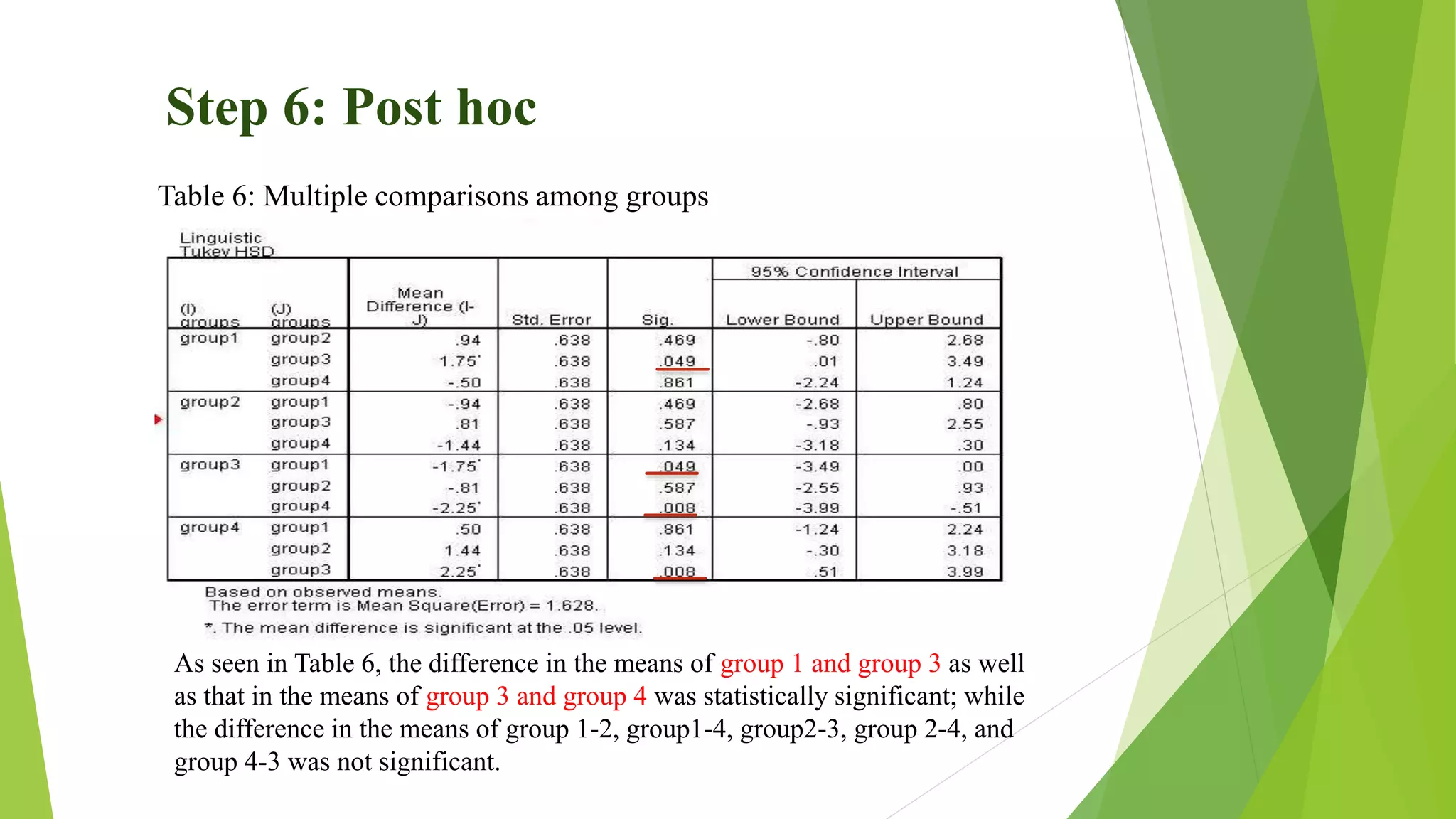
Table 6: Multiple comparisons among groups
As seen in Table 6, the difference in the means of group 1 and group 3 as well
as that in the means of group 3 and group 4 was statistically significant; while
the difference in the means of group 1-2, group1-4, group2-3, group 2-4, and
group 4-3 was not significant.

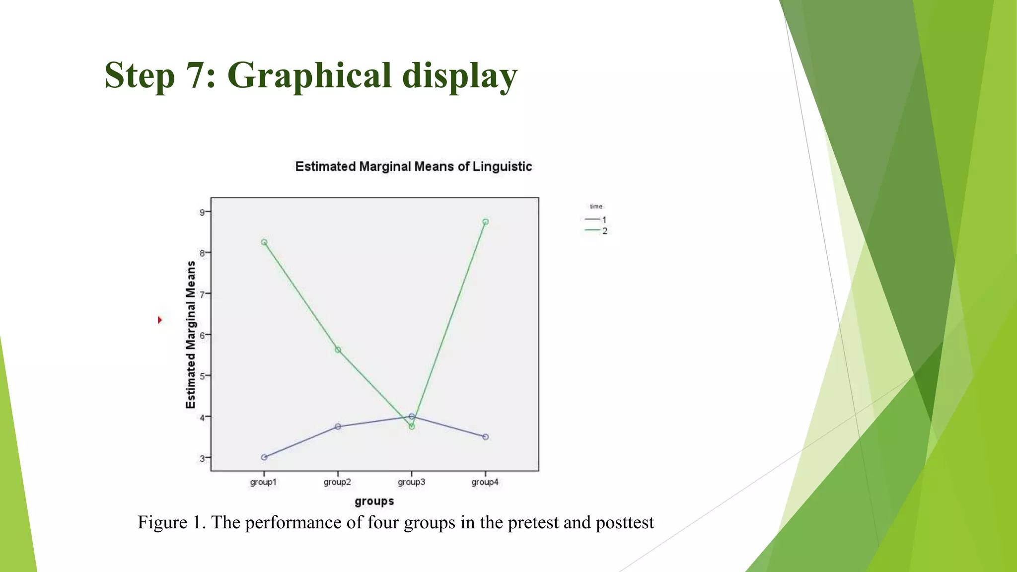
16. Step 7: Graphical display
Figure 1. The performance of four groups in the pretest and posttest