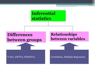
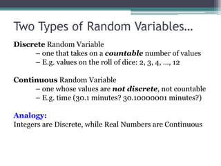
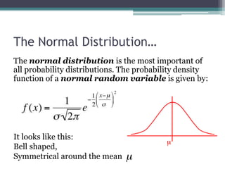
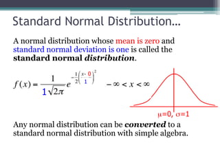
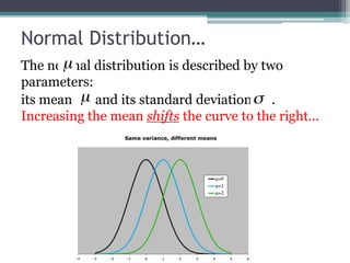
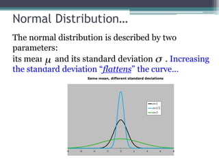
This document discusses quantitative research methods and statistical inference. It covers topics like probability distributions, sampling distributions, estimation, hypothesis testing, and different statistical tests. Key points include: - Probability distributions describe random variables and their associated probabilities. The normal distribution is important and described by its mean and standard deviation. 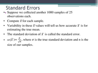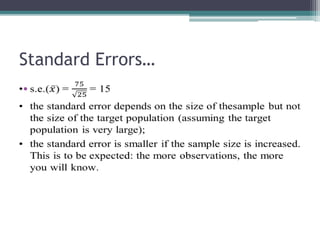- Sampling distributions allow making inferences about populations based on samples. The sampling distribution of the mean approximates a normal distribution as the sample size increases. 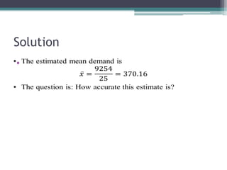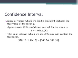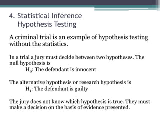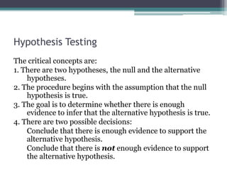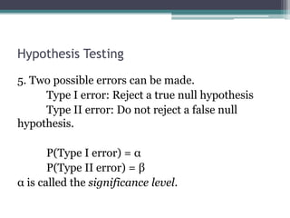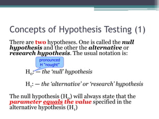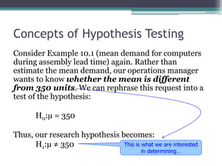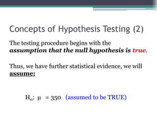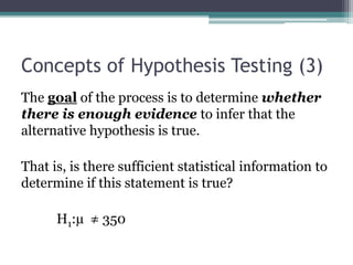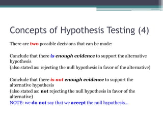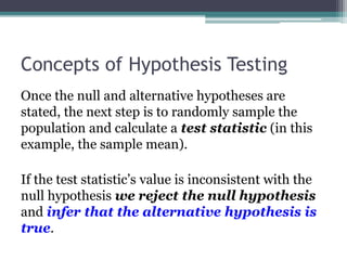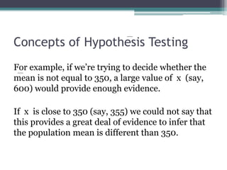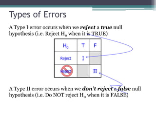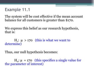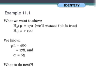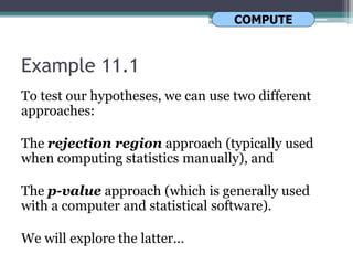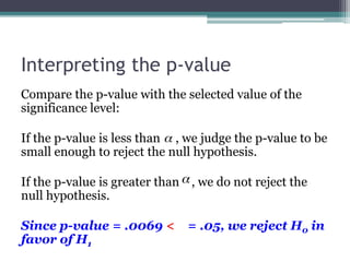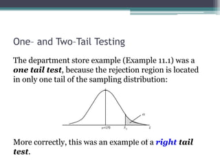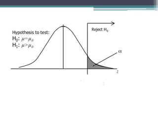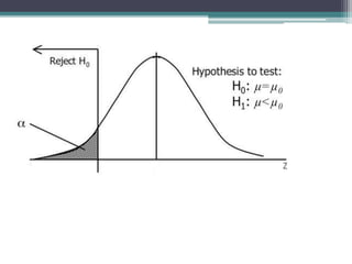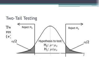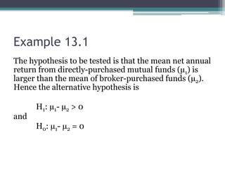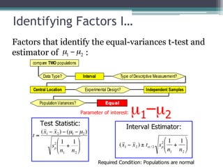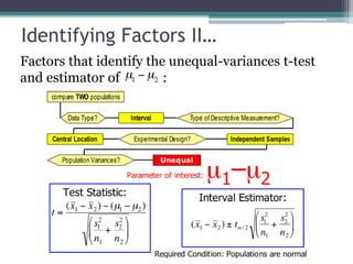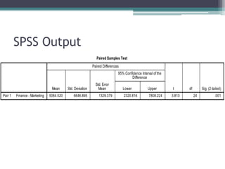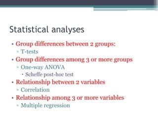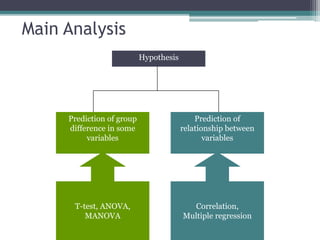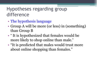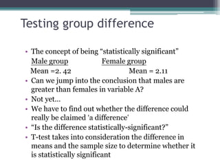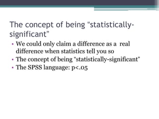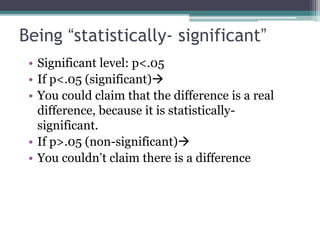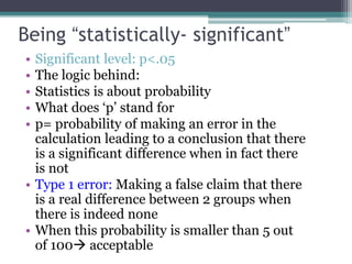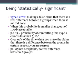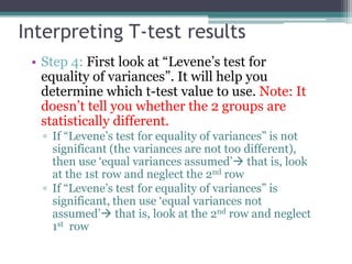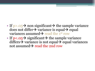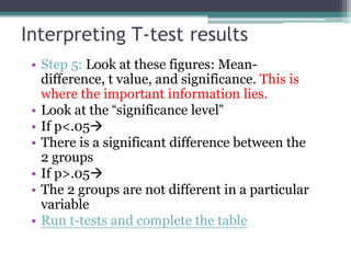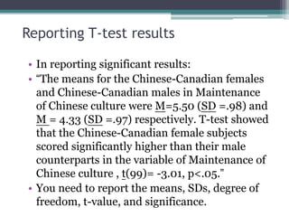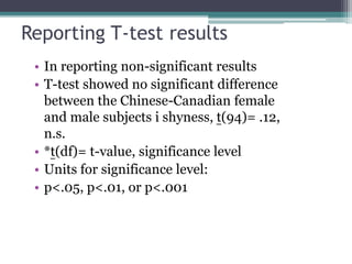- Statistical inference involves estimation and hypothesis testing. Estimation provides a value for an unknown population parameter based on a sample statistic. Hypothesis testing compares a null hypothesis to an alternative hypothesis based on a test statistic and can result in type 1 or type 2 errors.

1. Quantitative Research Methods
Lecture 6
1. Probability distribution
2. Sample distribution
3. Estimation
4. Hypothesis Testing
5. T-test

2. Inferential
statistics
Differences
between groups
Relationships
between variables
T-test, ANOVA, MANOVA Correlation, Multiple Regression

3. Review 2: Statistical Inference…
Statistical inference is the process by which we
acquire information and draw conclusions about
populations from samples.
In order to do inference, we require the skills and
knowledge of descriptive statistics, probability
distributions, and sampling distributions.

4. 1.Probability distribution…
• … is a table, formula, or graph that describes the
value of a random variable and the probability
associate with these values.

5. 1. Probability distribution:
Random Variables…
A random variable is a function or rule that
assigns a number to each outcome of an
experiment.
Alternatively, the value of a random variable is a
numerical event.
Instead of talking about the coin flipping event as
{heads, tails} think of it as
“the number of heads when flipping a coin”
{0, 1, 2…} (numerical events)

6. Two Types of Random Variables…
Discrete Random Variable
– one that takes on a countable number of values
– E.g. values on the roll of dice: 2, 3, 4, …, 12
Continuous Random Variable
– one whose values are not discrete, not countable
– E.g. time (30.1 minutes? 30.10000001 minutes?)
Analogy:
Integers are Discrete, while Real Numbers are Continuous

7. The Normal Distribution…
The normal distribution is the most important of
all probability distributions. The probability density
function of a normal random variable is given by:
It looks like this:
Bell shaped,
Symmetrical around the mean

8. Standard Normal Distribution…
A normal distribution whose mean is zero and
standard normal deviation is one is called the
standard normal distribution.
Any normal distribution can be converted to a
standard normal distribution with simple algebra.
0
1
1

9. Normal Distribution…
The normal distribution is described by two
parameters:
its mean and its standard deviation .
Increasing the mean shifts the curve to the right…

10. Normal Distribution…
The normal distribution is described by two
parameters:
its mean and its standard deviation . Increasing
the standard deviation “flattens” the curve…

11. 2. Sampling Distributions
The sampling distribution of the mean of a random
sample drawn from any population is
approximately normal for a sufficiently
large sample size.
The larger the sample size, the more closely the
sampling distribution of X will resemble a normal
distribution.

12. 3. Statistical Inference
Estimation
There are two types of inference: estimation and
hypothesis testing; estimation is introduced first.
The objective of estimation is to determine the
approximate value of a population parameter
on the basis of a sample statistic.
E.g., the sample mean ( ) is employed to
estimate the population mean ( ).

13. Estimation…
The objective of estimation is to determine the
approximate value of a population parameter
on the basis of a sample statistic.
There are two types of estimators:
Point Estimator
Interval Estimator

14. Point Estimator…
A point estimator draws inferences about a
population by estimating the value of an unknown
parameter using a single value or point.

15. Example Xm10-01
To lower costs, the operations manager wants to
use an inventory model. He notes demand during
lead time is normally distributed and he needs to
know the mean to compute the optimum inventory
level.
He observes 25 lead time periods and records the
demand during each period.
Assume that the manager knows that the standard
deviation is 75 computers.

16. Data
235 374 309 499 253
421 361 514 462 369
394 439 348 344 330
261 374 302 466 535
386 316 296 332 334

17. Solution
•

18. Standard Errors
•

19. Standard Errors…
•

20. Confidence Interval
•

21. Confidence Intervals…
• The 95% CI of the mean is the range of values
that will contain the true mean with a probability
of 0.95.
• Other CIs can be calculated by replacing 1.96 by a
different multiplying factor.
• The multiplying factor depends on the number of
observations in the sample and the confidence
level required.
• As the confidence level increases, so does the
multiplying factor.

22. 4. Statistical Inference
Hypothesis Testing
A criminal trial is an example of hypothesis testing
without the statistics.
In a trial a jury must decide between two hypotheses. The
null hypothesis is
H0: The defendant is innocent
The alternative hypothesis or research hypothesis is
H1: The defendant is guilty
The jury does not know which hypothesis is true. They must
make a decision on the basis of evidence presented.

23. 4. Statistical Inference
Hypothesis Testing
In the language of statistics convicting the
defendant is called
rejecting the null hypothesis in favor of the
alternative hypothesis.
That is, the jury is saying that there is enough
evidence to conclude that the defendant is guilty
(i.e., there is enough evidence to support the
alternative hypothesis).

24. 4. Statistical Inference
Hypothesis Testing
If the jury acquits it is stating that
there is not enough evidence to support the
alternative hypothesis.
Notice that the jury is not saying that the defendant is
innocent, only that there is not enough evidence to
support the alternative hypothesis. That is why we
never say that we accept the null hypothesis.

25. 4. Statistical Inference
Hypothesis Testing
There are two possible errors.
A Type I error occurs when we reject a true null
hypothesis. That is, a Type I error occurs when the
jury convicts an innocent person.
A Type II error occurs when we don’t reject a false
null hypothesis. That occurs when a guilty
defendant is acquitted.

26. 4. Statistical Inference
Hypothesis Testing
The probability of a Type I error is denoted as α
(Greek letter alpha). The probability of a type II
error is β (Greek letter beta).
The two probabilities are inversely related.
Decreasing one increases the other.

27. Hypothesis Testing
In our judicial system Type I errors are regarded as
more serious. We try to avoid convicting innocent
people. We are more willing to acquit guilty people.

28. Hypothesis Testing
The critical concepts are:
1. There are two hypotheses, the null and the alternative
hypotheses.
2. The procedure begins with the assumption that the null
hypothesis is true.
3. The goal is to determine whether there is enough
evidence to infer that the alternative hypothesis is true.
4. There are two possible decisions:
Conclude that there is enough evidence to support the
alternative hypothesis.
Conclude that there is not enough evidence to support
the alternative hypothesis.

29. Hypothesis Testing
5. Two possible errors can be made.
Type I error: Reject a true null hypothesis
Type II error: Do not reject a false null
hypothesis.
P(Type I error) = α
P(Type II error) = β
α is called the significance level.

30. Concepts of Hypothesis Testing (1)
There are two hypotheses. One is called the null
hypothesis and the other the alternative or
research hypothesis. The usual notation is:
H0: — the ‘null’ hypothesis
H1: — the ‘alternative’ or ‘research’ hypothesis
The null hypothesis (H0) will always state that the
parameter equals the value specified in the
alternative hypothesis (H1)
pronounced
H “nought”

31. Concepts of Hypothesis Testing
Consider Example 10.1 (mean demand for computers
during assembly lead time) again. Rather than
estimate the mean demand, our operations manager
wants to know whether the mean is different
from 350 units. We can rephrase this request into a
test of the hypothesis:
H0:µ = 350
Thus, our research hypothesis becomes:
H1:µ ≠ 350 This is what we are interested
in determining…

32. Concepts of Hypothesis Testing (2)
The testing procedure begins with the
assumption that the null hypothesis is true.
Thus, we have further statistical evidence, we will
assume:
H0: µ = 350 (assumed to be TRUE)

33. Concepts of Hypothesis Testing (3)
The goal of the process is to determine whether
there is enough evidence to infer that the
alternative hypothesis is true.
That is, is there sufficient statistical information to
determine if this statement is true?
H1:µ ≠ 350

34. Concepts of Hypothesis Testing (4)
There are two possible decisions that can be made:
Conclude that there is enough evidence to support the alternative
hypothesis
(also stated as: rejecting the null hypothesis in favor of the alternative)
Conclude that there is not enough evidence to support the
alternative hypothesis
(also stated as: not rejecting the null hypothesis in favor of the
alternative)
NOTE: we do not say that we accept the null hypothesis…

35. Concepts of Hypothesis Testing
Once the null and alternative hypotheses are
stated, the next step is to randomly sample the
population and calculate a test statistic (in this
example, the sample mean).
If the test statistic’s value is inconsistent with the
null hypothesis we reject the null hypothesis
and infer that the alternative hypothesis is
true.

36. Concepts of Hypothesis Testing
For example, if we’re trying to decide whether the
mean is not equal to 350, a large value of x (say,
600) would provide enough evidence.
If x is close to 350 (say, 355) we could not say that
this provides a great deal of evidence to infer that
the population mean is different than 350.

37. Types of Errors
A Type I error occurs when we reject a true null
hypothesis (i.e. Reject H0 when it is TRUE)
A Type II error occurs when we don’t reject a false null
hypothesis (i.e. Do NOT reject H0 when it is FALSE)
H0 T F
Reject I
Reject II

38. Example 11.1
The manager of a department store is thinking about
establishing a new billing system for the store's credit customers.
She determines that the new system will be cost-effective only if
the mean monthly account is more than $170. A random sample
of 400 monthly accounts is drawn, for which the sample mean is
$178.
The manager knows that the accounts are approximately
normally distributed with a standard deviation of $65. Can the
manager conclude from this that the new system will be cost-
effective?

39. Example 11.1
The system will be cost effective if the mean account
balance for all customers is greater than $170.
We express this belief as our research hypothesis,
that is:
H1: µ > 170 (this is what we want to
determine)
Thus, our null hypothesis becomes:
H0: µ = 170 (this specifies a single value for
the parameter of interest)

40. Example 11.1
What we want to show:
H0: µ = 170 (we’ll assume this is true)
H1: µ > 170
We know:
n = 400,
= 178, and
σ = 65
What to do next?!
IDENTIFY

41. Example 11.1
To test our hypotheses, we can use two different
approaches:
The rejection region approach (typically used
when computing statistics manually), and
The p-value approach (which is generally used
with a computer and statistical software).
We will explore the latter…
COMPUTE

42. p-Value of a Test
The p-value of a test is the probability of observing a
test statistic at least as extreme as the one computed
given that the null hypothesis is true.
In the case of our department store example, what is
the probability of observing a sample mean at least
as extreme as the one already observed (i.e. = 178),
given that the null hypothesis (H0: µ = 170) is true?
p-value

43. P-Value of a Test
p-value = P(Z > 2.46)
p-value =.0069
z =2.46

44. Interpreting the p-value
Overwhelming Evidence
(Highly Significant)
Strong Evidence
(Significant)
Weak Evidence
(Not Significant)
No Evidence
(Not Significant)
0 .01 .05 .10
p=.0069

45. Interpreting the p-value
Compare the p-value with the selected value of the
significance level:
If the p-value is less than , we judge the p-value to be
small enough to reject the null hypothesis.
If the p-value is greater than , we do not reject the
null hypothesis.
Since p-value = .0069 < = .05, we reject H0 in
favor of H1

46. One– and Two–Tail Testing
The department store example (Example 11.1) was a
one tail test, because the rejection region is located
in only one tail of the sampling distribution:
More correctly, this was an example of a right tail
test.

47. Right-Tail Testing

48. Left-Tail Testing

49. Two–Tail Testing
Two tail testing is used when we want to test a
research hypothesis that a parameter is not equal
(≠) to some value

50. Inferential
statistics
Differences
between groups
Relationships
between variables
T-test, ANOVA, MANOVA Correlation, Multiple Regression

51. 5. Two-Sample T-Test
Example 13.1 Xm13-01
Millions of investors buy mutual funds choosing from
thousands of possibilities.
Some funds can be purchased directly from banks or other
financial institutions while others must be purchased
through brokers, who charge a fee for this service.
This raises the question, can investors do better by buying
mutual funds directly than by purchasing mutual funds
through brokers.

52. Example 13.1 Xm13-01
To help answer this question a group of
researchers randomly sampled the annual returns
from mutual funds that can be acquired directly
and mutual funds that are bought through brokers
and recorded the net annual returns, which are the
returns on investment after deducting all relevant
fees.
Can we conclude at the 5% significance level that
directly-purchased mutual funds outperform
mutual funds bought through brokers?

53. Example 13.1
To answer the question we need to compare the
population of returns from direct and the returns
from broker- bought mutual funds.
The data are obviously interval (we've recorded
real numbers).

54. Example 13.1
The hypothesis to be tested is that the mean net annual
return from directly-purchased mutual funds (µ1) is
larger than the mean of broker-purchased funds (µ2).
Hence the alternative hypothesis is
H1: µ1- µ2 > 0
and
H0: µ1- µ2 = 0

55. Identifying Factors I…
Factors that identify the equal-variances t-test and
estimator of :

56. Identifying Factors II…
Factors that identify the unequal-variances t-test
and estimator of :

57. Using SPSS

58. Using SPSS

59. SPSS Output

60. The value of the test statistic is 2.29. The one-tail
p-value is .0122.
We observe that the p-value of the test is small.
As a result we conclude that there is sufficient
evidence to infer that on average directly-
purchased mutual funds outperform broker-
purchased mutual funds
Conclusion

61. Checking the Required Condition
Both the equal-variances and unequal-variances
techniques require that the populations be
normally distributed.

62. Example 13.4
In the last few years a number of web-based companies
that offer job placement services have been created.
The manager of one such company wanted to
investigate the job offers recent MBAs were obtaining.
In particular, she wanted to know whether finance
majors were being offered higher salaries than
marketing majors.

63. Example 13.4
In a preliminary study she randomly sampled 50
recently graduated MBAs half of whom majored in
finance and half in marketing.
From each, she obtained the highest salary
(including benefits) offer (Xm13-04).
Can we infer that finance majors obtain higher
salary offers than do marketing majors among
MBAs?

64. Example 13.4
The parameter is the difference between two
means (where µ1 = mean highest salary offer to
finance majors and µ2 = mean highest salary offer
to marketing majors).
Because we want to determine whether finance
majors are offered higher salaries, the alternative
hypothesis will specify that is greater than.

65. Example 13.4
The hypotheses are
0)(:H 210 
0)(:H 211 

66. Example 13.5
Suppose now that we redo the experiment in the
following way.
We examine the transcripts of finance and marketing
MBA majors.
We randomly sample a finance and a marketing major
whose grade point average (GPA) falls between 3.92
and 4 (based on a maximum of 4).
We then randomly sample a finance and a marketing
major whose GPA is between 3.84 and 3.92.

67. Example 13.5
We continue this process until the 25th pair of finance
and marketing majors are selected whose GPA fell
between 2.0 and 2.08.
(The minimum GPA required for graduation is 2.0.)
As we did in Example 13.4, we recorded the highest
salary offer . Xm13-05
Can we conclude from these data that finance majors
draw larger salary offers than do marketing majors?

68. Paired t-test
The experiment described in Example 13.4 is one in which
the samples are independent. That is, there is no
relationship between the observations in one sample and
the observations in the second sample. However, in this
example the experiment was designed in such a way that
each observation in one sample is matched with an
observation in the other sample. The matching is conducted
by selecting finance and marketing majors with similar
GPAs. Thus, it is logical to compare the salary offers for
finance and marketing majors in each group. This type of
experiment is called matched pairs.

69. Example 13.5
For each GPA group, we calculate the matched pair
difference between the salary offers for finance and
marketing majors.

70. Example 13.5
The numbers in black are the original starting salary
data (Xm13-05) ; the numbers in blue were calculated.
although a student is either in Finance OR
in Marketing (i.e. independent), that the
data is grouped in this fashion makes it a
matched pairs experiment (i.e. the two
students in group #1 are ‘matched’ by
their GPA range
the difference of the means is equal to the mean of the differences, hence
we will consider the “mean of the paired differences” as our parameter of interest:
IDENTIFY

71. Example 13.5
Do Finance majors have higher salary offers than Marketing
majors?
Since:
We want to research this hypothesis: H1:
(and our null hypothesis becomes H0: )
IDENTIFY

72. Test Statistic for
The test statistic for the mean of the
population of differences ( ) is:
which is Student t distributed with nD–1 degrees of
freedom, provided that the differences are
normally distributed.
IDENTIFY

73. Using SPSS
Analyze > Compare Means > Paired Samples T
Test

74. SPSS Output

75. Example 13.5
The p-value is .0004. There is overwhelming
evidence that Finance majors do obtain higher
starting salary offers than their peers in Marketing.

76. Statistical analyses
• Group differences between 2 groups:
▫ T-tests
• Group differences among 3 or more groups
▫ One-way ANOVA
 Scheffe post-hoc test
• Relationship between 2 variables
▫ Correlation
• Relationship among 3 or more variables
▫ Multiple regression

77. Main Analysis
Hypothesis
Prediction of
relationship between
variables
Prediction of group
difference in some
variables
T-test, ANOVA,
MANOVA
Correlation,
Multiple regression

78. Hypotheses regarding group
difference
• The hypothesis language
• Group A will be more (or less) in (something)
than Group B
• “ It is hypothesized that females would be
more likely to shop online than male.”
• “It is predicted that males would trust more
about online shopping than females.”

79. Testing group difference
• Comparing 2 groups’ difference in some
variables
• We use Independent-samples t-test
Male group Female group
Subj.1 Subj. 1
2 2
3 3
4 4
• Note: t-tests can compare only 2 groups at a
time

80. Comparing males and females on
these variables
Degree of enjoyment on online shopping M > F

81. Variable Female Male
Variable A
Testing group difference

82. Testing group difference
• The concept of being “statistically significant”
Male group Female group
Mean =2. 42 Mean = 2.11
• Can we jump into the conclusion that males are
greater than females in variable A?
• Not yet…
• We have to find out whether the difference could
really be claimed ‘a difference’
• “Is the difference statistically-significant?”
• T-test takes into consideration the difference in
means and the sample size to determine whether it
is statistically significant

83. The concept of being “statistically-
significant”
• We could only claim a difference as a real
difference when statistics tell you so
• The concept of being “statistically-significant”
• The SPSS language: p<.05

84. Being “statistically- significant”
• Significant level: p<.05
• If p<.05 (significant)
• You could claim that the difference is a real
difference, because it is statistically-
significant.
• If p>.05 (non-significant)
• You couldn’t claim there is a difference

85. Being “statistically- significant”
• Significant level: p<.05
• The logic behind:
• Statistics is about probability
• What does ‘p’ stand for
• p= probability of making an error in the
calculation leading to a conclusion that there
is a significant difference when in fact there
is not
• Type 1 error: Making a false claim that there
is a real difference between 2 groups when
there is indeed none
• When this probability is smaller than 5 out
of 100 acceptable

86. Being “statistically- significant”
• Type 1 error: Making a false claim that there is a
real difference between 2 groups when there is
indeed none
• When this probability is smaller than 5 out of
100 acceptable
• p<.05 = probability of committing this Type 1
error is less than 5/100
• Over 95% of the time when you make the claim
that there is a difference between the groups in
certain aspects, you are correct
• p> .05 not acceptable, no real difference
between 2 groups.

87. Running T-tests
• Steps for running a t-test:
• Analyze
Compare means
Independent-sample T-test
Grouping variables
Define (which two
groups)
Testing variables

88. Running T-tests
• Task: Perform t-tests to see if there is any gender
difference in income GSS2008 data.

89. Interpreting T-test results
• T-test output
• 1) Look at the means of the 2 groups (To
see which group has a higher mean)
• 2) Look at ‘Levene’s test of equality of
variance’:
• If non-significant> no significant different
in the variance> equal variance> rely on
the top row

90. Interpreting T-test results
• T-test output
• Step 1: The output from the t-test procedure
is segmented by two parts: variables and
types of information.
• Step 2: For each dependent variable, SPSS
reports descriptive statistics in the first part.
Look at the means of the 2 groups (To see
which group has a higher mean than the
other in a variable)
• Step 3: To see if there is significant
difference. We need to make reference to
part 2:

91. Interpreting T-test results
• Step 4: First look at “Levene’s test for
equality of variances”. It will help you
determine which t-test value to use. Note: It
doesn’t tell you whether the 2 groups are
statistically different.
▫ If “Levene’s test for equality of variances” is not
significant (the variances are not too different),
then use ‘equal variances assumed’ that is, look
at the 1st row and neglect the 2nd row
▫ If “Levene’s test for equality of variances” is
significant, then use ‘equal variances not
assumed’ that is, look at the 2nd row and neglect
1st row

92. • If p>.05 non significant the sample variance
does not differ variance is equal equal
variances assumed read the 1st row
• If p<.05 significant the sample variance
differs variance is not equal equal variances
not assumed read the 2nd row

93. Interpreting T-test results
• Step 5: Look at these figures: Mean-
difference, t value, and significance. This is
where the important information lies.
• Look at the “significance level”
• If p<.05
• There is a significant difference between the
2 groups
• If p>.05
• The 2 groups are not different in a particular
variable
• Run t-tests and complete the table

94. Reporting T-test results
• In reporting significant results:
• “The means for the Chinese-Canadian females
and Chinese-Canadian males in Maintenance
of Chinese culture were M=5.50 (SD =.98) and
M = 4.33 (SD =.97) respectively. T-test showed
that the Chinese-Canadian female subjects
scored significantly higher than their male
counterparts in the variable of Maintenance of
Chinese culture , t(99)= -3.01, p<.05.”
• You need to report the means, SDs, degree of
freedom, t-value, and significance.

95. Reporting T-test results
• In reporting non-significant results
• T-test showed no significant difference
between the Chinese-Canadian female
and male subjects i shyness, t(94)= .12,
n.s.
• *t(df)= t-value, significance level
• Units for significance level:
• p<.05, p<.01, or p<.001

96. Week 3 Assignment
• Read chapter 9-13
• Assignment: