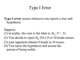
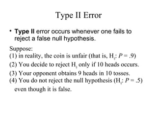
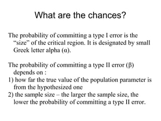
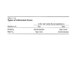
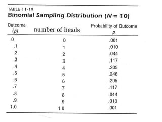
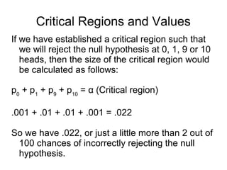
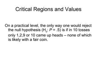
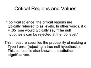
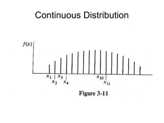
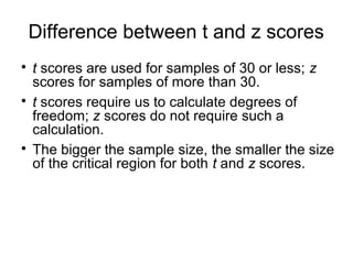
1) The document discusses hypothesis testing and statistical inference using examples related to coin tossing. It explains the concepts of type I and type II errors and how hypothesis tests are conducted.
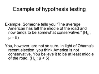
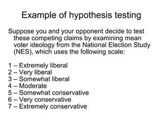
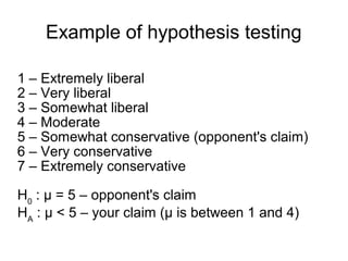
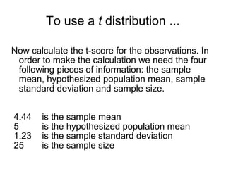
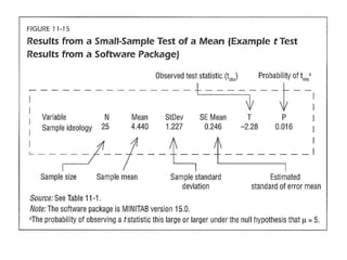
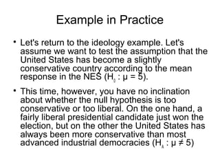
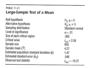
2) An example is provided to test the hypothesis that the average American ideology is somewhat conservative (H0: μ = 5) using data from the National Election Study. The alternative hypothesis is that the average is less than 5 (HA: μ < 5).
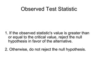
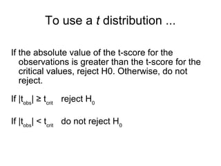
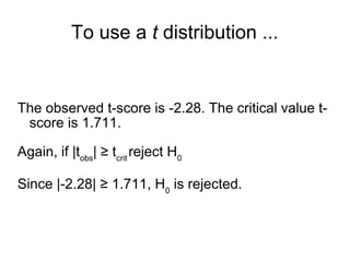
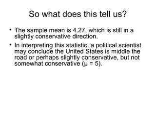
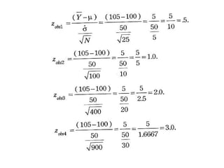
3) The results of the hypothesis test show the observed test statistic is lower than the critical value, so the null hypothesis that the average is 5 is rejected in favor of the alternative that the average is less than 5.

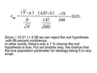


![Getting Started with Apache Spark: Big Data Made Simple [Free Meetup]](https://cdn.slidesharecdn.com/ss_thumbnails/apachesparkgettingstarted-260203175547-8361bcc3-thumbnail.jpg?width=640&height=640&fit=bounds)


