7 anova chi square test

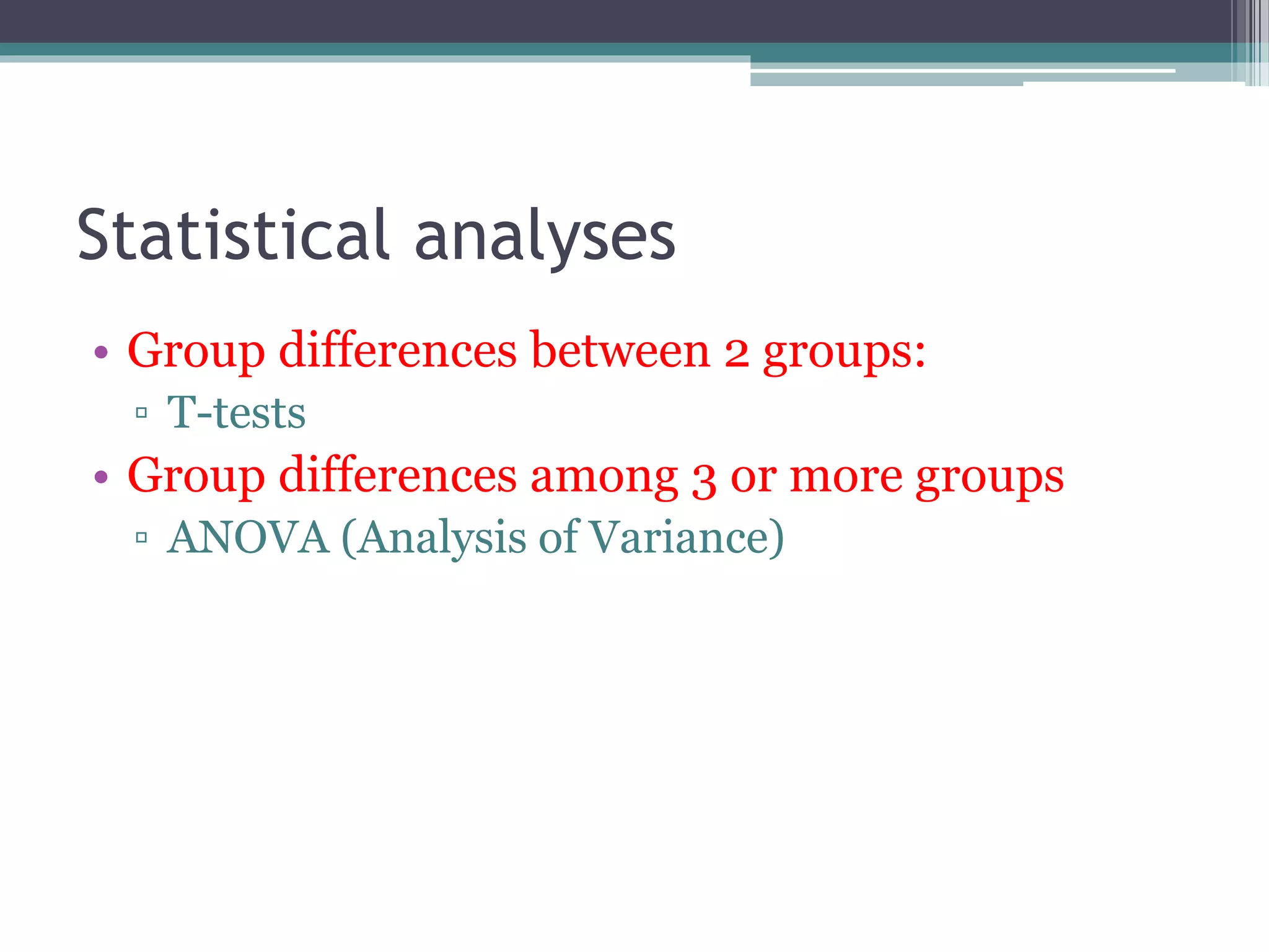
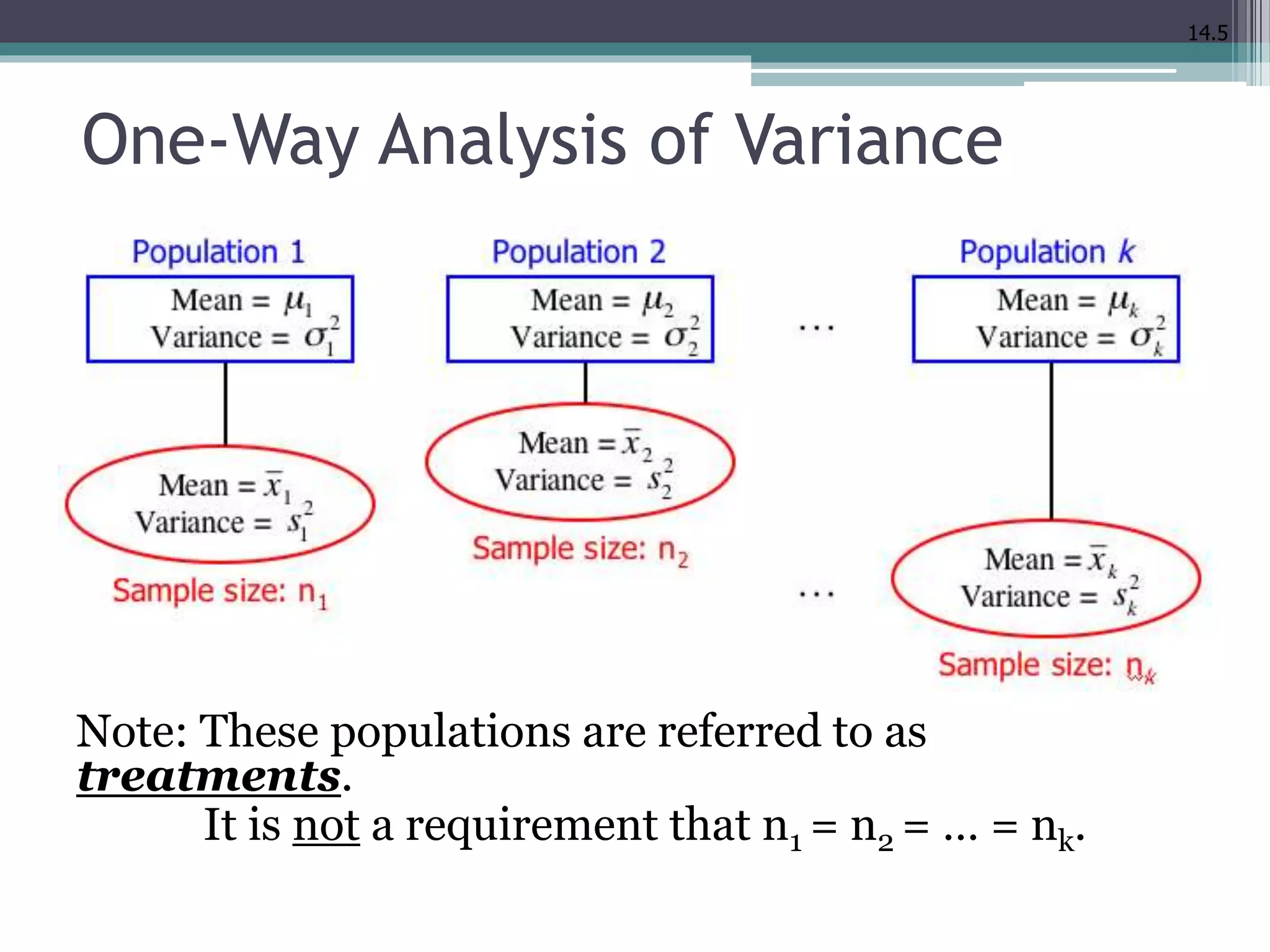
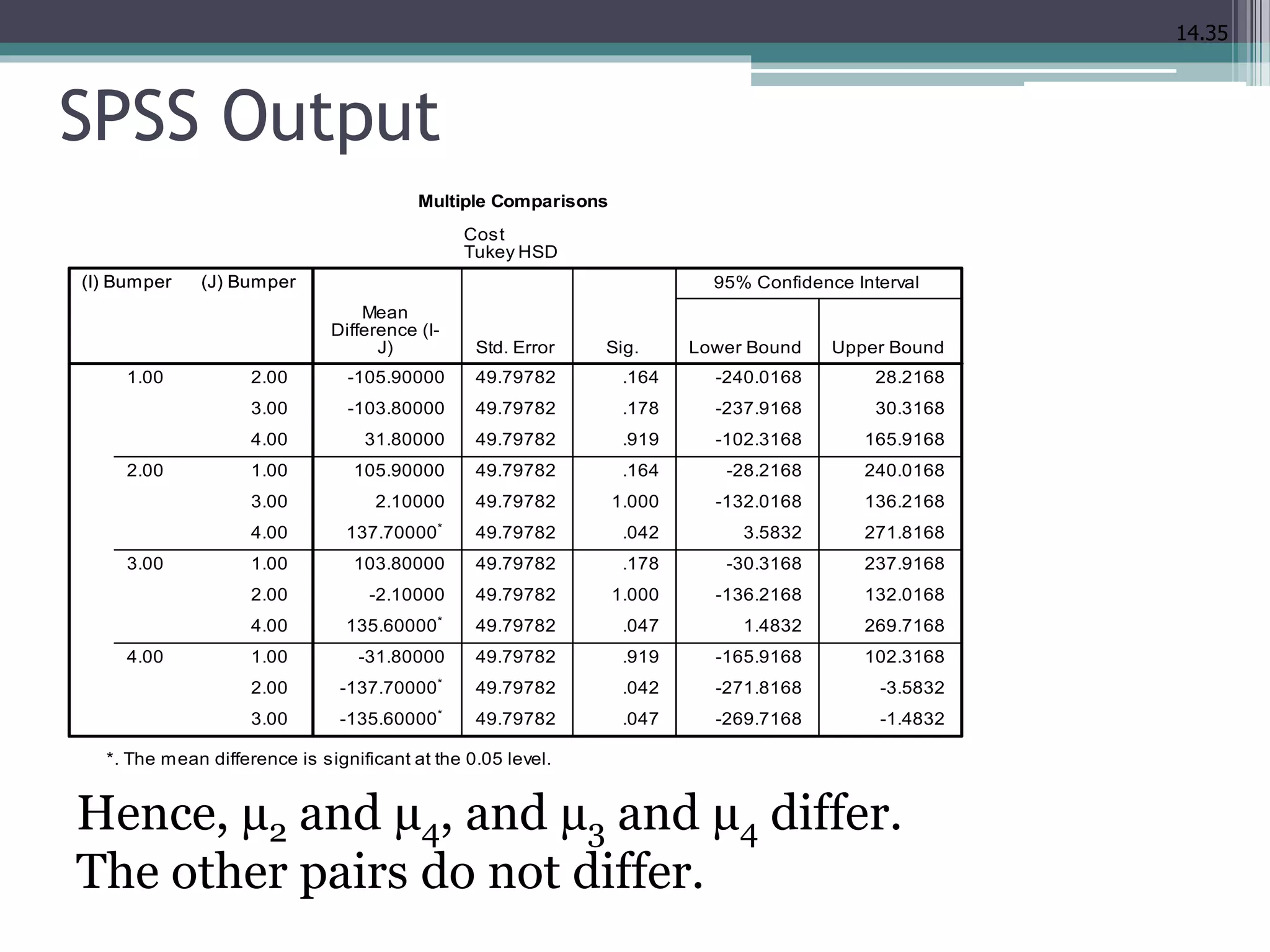
Quantitative Research Methods
Lecture 7
1. ANOVA:
One-way ANOVA,
Two-way ANOVA
Two factor ANOVA
2. Chi-Squared Tests

Inferential
statistics
Differences
between groups
Relationships
between variables
T-test, ANOVA, MANOVA Correlation, Multiple Regression

Statistical analyses
• Group differences between 2 groups:
▫ T-tests
• Group differences among 3 or more groups
▫ ANOVA (Analysis of Variance)

Analysis of Variance
Analysis of variance is a technique that allows us
to compare three or more populations of interval
data.
Analysis of variance is:
 an extremely powerful and widely used
procedure.
 a procedure which determines whether
differences exist between population means.
 a procedure which works by analyzing
sample variance.

14.5
One-Way Analysis of Variance
Independent samples are drawn from k populations:
Note: These populations are referred to as
treatments.
It is not a requirement that n1 = n2 = … = nk.

14.6
One Way Analysis of Variance
New Terminology:
x is the response variable, and its values are
responses.
xij refers to the ith observation in the jth sample.
E.g. x35 is the third observation of the fifth sample.
The grand mean, , is the mean of all the observations,
i.e.:
(n = n1 + n2 + … + nk)

14.7
One Way Analysis of Variance
More New Terminology:
Population classification criterion is called a
factor.
Each population is a factor level.

14.8
Example 14.1
In the last decade stockbrokers have drastically
changed the way they do business. It is now easier and
cheaper to invest in the stock market than ever before.
What are the effects of these changes?
To help answer this question a financial analyst
randomly sampled 366 American households and
asked each to report the age of the head of the
household and the proportion of their financial assets
that are invested in the stock market.

14.9
Example 14.1
The age categories are
Young (Under 35)
Early middle-age (35 to 49)
Late middle-age (50 to 65)
Senior (Over 65)
The analyst was particularly interested in determining
whether the ownership of stocks varied by age. Xm14-
01
Do these data allow the analyst to determine that there
are differences in stock ownership between the four
age groups?

14.10
Example 14.1
Percentage of total assets invested in the stock
market is the response variable; the actual
percentages are the responses in this example.
Population classification criterion is called a factor.
The age category is the factor we’re interested in.
This is the only factor under consideration (hence
the term “one way” analysis of variance).
Each population is a factor level.
In this example, there are four factor levels: Young,
Early middle age, Late middle age, and Senior.
Terminology

14.11
Example 14.1
The null hypothesis in this case is:
H0:µ1 = µ2 = µ3 = µ4
i.e. there are no differences between population
means.
Our alternative hypothesis becomes:
H1: at least two means differ
OK. Now we need some test statistics…

14.12
Test Statistic
Since µ1 = µ2 = µ3 = µ4 is of interest to us, a statistic that
measures the proximity of the sample means to each
other would also be of interest.
Such a statistic exists, and is called the between-
treatments variation. It is denoted SST, short for “sum
of squares for treatments”. Its is calculated as:
grand mean
sum across k treatments
A large SST indicates large variation between sample means which supports H1.

14.13
Test Statistic
SST gave us the between-treatments variation. A
second statistic, SSE (Sum of Squares for Error)
measures the within-treatments variation.
SSE is given by: or:
In the second formulation, it is easier to see that it
provides a measure of the amount of variation
we can expect from the random variable we’ve
observed.

14.14
Example 14.1
Since:
If it were the case that:
then SST = 0 and our null hypothesis, H0:µ1 = µ2 = µ3 = µ4
would be supported.
More generally, a small value of SST supports the
null hypothesis. A large value of SST supports the
alternative hypothesis. The question is, how large
is “large enough”?
4321 xxxx 

14.15
Mean Squares
The mean square for treatments (MST) is given by:
The mean square for errors (MSE) is given by:
And the test statistic:
is F-distributed with k–1 and n–k degrees of
freedom.

14.16
Example 14.1
Since the purpose of calculating the F-statistic is to
determine whether the value of SST is large
enough to reject the null hypothesis, if SST is
large, F will be large.
P-value = P(F > Fstat)

Example 14.1 SPSS
• Analyze  Compare Means  One-way ANOVA

14.19
Example 14.1
Since the p-value is .041, which is small we reject the
null hypothesis (H0:µ1 = µ2 = µ3 = µ4) in favor of the
alternative hypothesis (H1: at least two population
means differ).
That is: there is enough evidence to infer that the mean
percentages of assets invested in the stock market
differ between the four age categories.

14.20
Identifying Factors
Factors that Identify the One-Way Analysis of
Variance:

14.21
Checking the Required Conditions
The F-test of the analysis of variance requires that
the random variable be normally distributed with
equal variances.
If the data are not normally distributed we can
replace the one-way analysis of variance with its
nonparametric counterpart, which is the Kruskal-
Wallis test.

To test normality:
• Analyze  Descriptive  Explore

Result of Normality test
• Check Shapiro-Wilk test, if p<.05, not
significant, not normally distributed; if p>.05,
significant, normally distributed
• Check shapes of histogram

14.24
Multiple Comparisons
When we conclude from the one-way analysis of
variance that at least two treatment means differ (i.e. we
reject the null hypothesis that H0: ), we often
need to know which treatment means are responsible for
these differences.
We will examine three statistical inference procedures that
allow us to determine which population means differ:
• Fisher’s least significant difference (LSD) method
• Bonferroni adjustment, and
• Tukey’s multiple comparison method.

14.25
Multiple Comparisons
Two means are considered different if the difference
between the corresponding sample means is larger
than a critical number. The general case for this is,
IF
THEN we conclude and differ.
The larger sample mean is then believed to be
associated with a larger population mean.

Post Hoc in SPSS
• Analyze  Compare Means  One-way
ANOVA Post Hoc  LSD/ Bonferroni/Tukey

14.28
Example 14.2
North American automobile manufacturers have become
more concerned with quality because of foreign competition.
One aspect of quality is the cost of repairing damage caused
by accidents. A manufacturer is considering several new
types of bumpers.
To test how well they react to low-speed collisions, 10
bumpers of each of four different types were installed on
mid-size cars, which were then driven into a wall at 5 miles
per hour.

14.29
Example 14.2
The cost of repairing the damage in each case was
assessed. Xm14-02
a Is there sufficient evidence to infer that the
bumpers differ in their reactions to low-speed
collisions?
b If differences exist, which bumpers differ?

Checking Required Assumptions
14.30

14.31
Example 14.2
The problem objective is to compare four populations, the
data are interval, and the samples are independent. The
correct statistical method is the one-way analysis of
variance.
F = 4.06, p-value = .0139. There is enough evidence to infer
that a difference exists between the four bumpers. The
question is now, which bumpers differ?
11
12
13
14
15
16
A B C D E F G
ANOVA
Source of Variation SS df MS F P-value F crit
Between Groups 150,884 3 50,295 4.06 0.0139 2.8663
Within Groups 446,368 36 12,399
Total 597,252 39

14.32
Using SPSS
Analyze > Compare means > One way ANOVA

Using SPSS (Homogeneity of Variance)
14.34

14.35
SPSS Output
Hence, µ2 and µ4, and µ3 and µ4 differ.
The other pairs do not differ.

14.36
Analysis of Variance Experimental
Designs
Experimental design determines which
analysis of variance technique we use.
One-way analysis of variance is only one of many
different experimental designs of the analysis of
variance.

14.37
Analysis of Variance Experimental
Designs
A multifactor experiment is one where there are two or
more factors that define the treatments.
For example, if instead of just varying the advertising
strategy for our new apple juice product we also varied the
advertising medium (e.g. television or newspaper), then we
have a two-factor analysis of variance situation.
The first factor, advertising strategy, still has three levels
(convenience, quality, and price) while the second factor,
advertising medium, has two levels (TV or print).

14.38
Independent Samples and Blocks
Similar to the ‘matched pairs experiment’, a
randomized block design experiment reduces the
variation within the samples, making it easier to
detect differences between populations.
The term block refers to a matched group of
observations from each population.
We can also perform a blocked experiment by using
the same subject for each treatment in a “repeated
measures” experiment.

14.39
Independent Samples and Blocks
The randomized block experiment is also called
the two-way analysis of variance, not to be
confused with the two-factor analysis of
variance. To illustrate where we’re headed…
we’ll
do this
first

14.40
Example 14.3
Many North Americans suffer from high levels of cholesterol,
which can lead to heart attacks. For those with very high levels
(over 280), doctors prescribe drugs to reduce cholesterol levels.
A pharmaceutical company has recently developed four such
drugs. To determine whether any differences exist in their
benefits, an experiment was organized. The company selected 25
groups of four men, each of whom had cholesterol levels in
excess of 280. In each group, the men were matched according to
age and weight. The drugs were administered over a 2-month
period, and the reduction in cholesterol was recorded (Xm14-
03). Do these results allow the company to conclude that
differences exist between the four new drugs?

14.41
Example 14.3
The hypotheses to test in this case are:
H0:µ1 = µ2 = µ3 = µ4
H1: At least two means differ

14.42
Example 14.3
Each of the four drugs can be considered a
treatment.
Each group can be blocked, because they are matched
by age and weight.
By setting up the experiment this way, we eliminate
the variability in cholesterol reduction related to
different combinations of age and weight. This helps
detect differences in the mean cholesterol reduction
attributed to the different drugs.

14.43
Example 14.3
Block
Treatment
There are b = 25 blocks, and
k = 4 treatments in this example.
Group Drug 1 Drug 2 Drug 3 Drug 4
1 6.6 12.6 2.7 8.7
2 7.1 3.5 2.4 9.3
3 7.5 4.4 6.5 10.0
4 9.9 7.5 16.2 12.6
5 13.8 6.4 8.3 10.6
6 13.9 13.5 5.4 15.4

14.44
Using SPSS
Analyze > General Linear Model > Univariate
>Model > Build terms/Custom

14.46
Checking the Required Conditions
The F-test of the randomized block design of the analysis
of variance has the same requirements as the independent
samples design.
That is, the random variable must be normally distributed
and the population variances must be equal.

14.47
Identifying Factors
Factors that Identify the Randomized Block of the
Analysis of Variance:

14.48
Violation of the Required Conditions
When the response is not normally distributed, we can
replace the randomized block analysis of variance with the
Friedman test.

14.49
Two-Factor Analysis of Variance…
• In factorial experiments, we can examine the effect
on the response variable of two or more factors.
• We can use the analysis of variance to determine
whether the levels of each factor are different from
one another.

14.50
Example 14.4
One measure of the health of a nation’s economy is how
quickly it creates jobs. One aspect of this issue is the
number of jobs individuals hold.
As part of a study on job tenure, a survey was conducted
wherein Americans aged between 37 and 45 were asked
how many jobs they have held in their lifetimes. Also
recorded were gender and educational attainment.

14.51
Example 14.4
The categories are
Less than high school (E1)
High school (E2)
Some college/university but no degree (E3)
At least one university degree (E4)
The data were recorded for each of the eight categories of
Gender and education. Xm14-04
Can we infer that differences exist between genders and
educational levels?

14.52
Example 14.4
Male E1 Male E2 Male E3 Male E4 Female E1 Female E2 Female E3 Female E4
10 12 15 8 7 7 5 7
9 11 8 9 13 12 13 9
12 9 7 5 14 6 12 3
16 14 7 11 6 15 3 7
14 12 7 13 11 10 13 9
17 16 9 8 14 13 11 6
13 10 14 7 13 9 15 10
9 10 15 11 11 15 5 15
11 5 11 10 14 12 9 4
15 11 13 8 12 13 8 11

14.53
Example 14.4
We begin by treating this example as a one-way
analysis of
variance with eight treatments.
However, the treatments are defined by two different
factors.
One factor is gender, which has two levels.
The second factor is educational attainment, which
has four levels.

14.54
Example 14.4
We can proceed to solve this problem in the same
way we did in Section 14.1: that is, we test the
following hypotheses:
H1: At least two means differ.
876543210 :H 

14.55
Using SPSS
• Analyze > General Linear Model > Univariate

14.56
Example 14.4
The value of the test statistic is F = 2.17 with a p-
value of .047.
We conclude that there are differences in the
number of jobs between the eight treatments.

14.57
Example 14.4
This statistical result raises more questions.
Namely, can we conclude that the differences in the mean
number of jobs are caused by differences between males and
females?
Or are they caused by differences between educational
levels?
Or, perhaps, are there combinations, called interactions of
gender and education that result in especially high or low
numbers?

14.58
Terminology
• A complete factorial experiment is an experiment in
which the data for all possible combinations of the levels of
the factors are gathered. This is also known as a two-way
classification.
• The two factors are usually labeled A & B, with the number of
levels of each factor denoted by a & b respectively.
• The observations for each combination are called
replicates, their number is denoted by r. For our purposes,
the number of replicates will be the same for each treatment,
that is they are balanced.

14.59
Terminology Xm14-04a
Male Female
Less than high school 10 7
9 13
12 14
16 6
14 11
17 14
13 13
9 11
11 14
15 12
High School 12 7
11 12
9 6
14 15
12 10
16 13
10 9
10 15
5 12
11 13
Less than Bachelor's degree 15 5
8 13
7 12
7 3
7 13
9 11
14 15
15 5
11 9
13 8
At least one Bachelor's degree 8 7
9 9
5 3
11 7
13 9
8 6
7 10
11 15
10 4
8 11

14.60
Terminology
• Thus, we use a complete factorial experiment
where the number of treatments is ab with r
replicates per treatment.
• In Example 14.4, a = 2, b = 4, and r = 10.
• As a result, we have 10 observations for each of
the eight treatments.

14.61
Example 14.4
If you examine the ANOVA table, you can see that the total
variation is SS(Total) = 879.55, the sum of squares for
treatments is SST = 153.35, and the sum of squares for error
is SSE = 726.20.
The variation caused by the treatments is measured by SST.
In order to determine whether the differences are due to
factor A, factor B, or some interaction between the two
factors, we need to partition SST into three sources.
These are SS(A), SS(B), and SS(AB).

14.62
Example 14.4
Test for the differences between the Levels of Factor
A…
H0: The means of the a levels of Factor A are equal
Test statistic: F = MS(A) / MSE
Example 14.4: Are there differences in the mean
number of jobs between men and women?
H0: µmen = µwomen

14.63
Example 14.4
Test for the differences between the Levels of Factor B…
H0: The means of the a levels of Factor B are equal
Test statistic: F = MS(B) / MSE
Example 14.4: Are there differences in the mean number of
jobs between the four educational levels?
4321 EEEE0 :H 

14.64
Example 14.4
Test for interaction between Factors A and B…
H0: Factors A and B do not interact to affect the mean
responses.
H1: Factors A and B do interact to affect the mean
responses.
Test statistic: F = MS(AB) / MSE
Example 14.4: Are there differences in the mean
number of jobs caused by interaction
between gender and educational level?

Levels of factor A
1 2 3
Level 1 of factor B
Level 2 of factor B
1 2 3
1 2 31 2 3
Level 1and 2 of factor B
Difference among the levels of factor A
No difference among the levels of factor B
Difference among the levels of factor A, and
difference among the levels of factor B; no
interaction
Levels of factor A
Levels of factor A Levels of factor A
No difference among the levels of factor A.
Difference among the levels of factor B
Interaction
M R
e s
a p
n o
n
s
e
M R
e s
a p
n o
n
s
e
M R
e s
a p
n o
n
s
e
M R
e s
a p
n o
n
s
e

14.66
Using SPSS
Analyze > General Linear Model > Univariate

14.67
Output
In the ANOVA table Sample refers to factor B educational
level) and Columns refers to factor A (gender). Thus, MS(B) =
45.28, MS(A) =11.25, MS(AB) = 2.08 and MSE = 10.09. The F-
statistics are 4.49 (educational level), 1.12 (gender), and .21
(interaction).

14.68
Example 14.4
There are significant differences between the
mean number of jobs held by people with different
educational backgrounds.
There is no difference between the mean number
of jobs held by men and women.
Finally, there is no interaction.

14.69
Identifying Factors…
• Independent Samples Two-Factor Analysis of Variance…

Review: 2.6. Hands on: Graphical
Descriptive Techniques I
Graphical
Techniques
Objective Data type Ex
Frequency and
Relative Frequency
(Proportion)
Tables
Bar charts
Pie Chart
Describe a single
set of data
Nominal or
ordinal
P18 GSS2008
P24
Xm02-02
P27
Ex2.11 Bar
Ex2.12 Pie
Cross-classification
Table
Cluster bar chats
Describe the
relationship
between two
variables and
compare two ore
more sets of data
Nominal P34
Xm02-04
P37
ANES2008

Chi-square test
• Objective: Analyze the relationship between two
nominal variable and compare two or more
populations.
• H0: The two variables are independent.
• H1: The two variables are dependent.
• E.g. P34. Xm02-04
• newspaper and occupation

SPSS
• Analyze> Descriptive> Crosstabs

SPSS
• Analyze> Descriptive> Crosstabs > statistics > Chi-square
(sig) and Phi and Cramer’s V (strength)

Example 15.2 data: Xm15-02
• Relationship between undergraduate degree and
MBA major
▫ Graphic
▫ Chi-square test

Summary
• ANOVA: two or more group difference on a
interval variable
• Chi-square test: relationship btw two nominal
variables

7 anova chi square test

More Related Content

What's hot

Similar to 7 anova chi square test

More from Penny Jiang

Recently uploaded

7 anova chi square test